Data Analytics Fundamentals
Data Analytics Fundamentals: From Raw Data to Actionable Insights
Introduction to Data Analytics
Data analytics is the systematic process of examining raw data to uncover meaningful patterns, correlations, and insights. In today's data-driven world, analytics transforms information into actionable knowledge that drives business decisions, operational improvements, and strategic planning.
The Evolution of Data Analytics
Historical Context:
- Descriptive Analytics: What happened? (Traditional reporting)
- Diagnostic Analytics: Why did it happen? (Root cause analysis)
- Predictive Analytics: What will happen? (Forecasting and modeling)
- Prescriptive Analytics: What should we do? (Optimization and recommendations)
Benefits of Data Analytics
Strategic Advantages:
- Informed Decision Making: Data-driven insights replace intuition and guesswork
- Operational Efficiency: Identify bottlenecks and optimization opportunities
- Risk Mitigation: Early detection of trends and potential issues
- Competitive Edge: Understanding market dynamics and customer behavior
- Cost Reduction: Eliminating waste and improving resource allocation
The Data Analytics Process
Effective data analytics follows a structured methodology that ensures comprehensive analysis and reliable results.
Core Components
1. Data Collection:
- Identifying relevant data sources
- Establishing data acquisition pipelines
- Ensuring data quality and completeness
2. Data Processing:
- Data cleaning and validation
- Transformation and normalization
- Integration of multiple data sources
3. Data Analysis:
- Exploratory data analysis (EDA)
- Statistical modeling and testing
- Pattern recognition and correlation analysis
4. Data Visualization:
- Creating meaningful charts and dashboards
- Communicating insights effectively
- Supporting data-driven storytelling
5. Action and Monitoring:
- Implementing insights into business processes
- Continuous monitoring and refinement
- Measuring impact and ROI
Analytical Frameworks
CRISP-DM (Cross-Industry Standard Process for Data Mining):
- Business Understanding
- Data Understanding
- Data Preparation
- Modeling
- Evaluation
- Deployment
TDSP (Team Data Science Process):
- Business Understanding
- Data Acquisition and Understanding
- Modeling
- Deployment
- Customer Acceptance## The 5Vs of Big Data
Modern data analytics must contend with the challenges and opportunities presented by big data characteristics.
Volume: Scale and Storage
Understanding Data Volume:
- Traditional Data: Structured databases, spreadsheets
- Big Data Volume: Petabytes to exabytes of information
- Growth Drivers: IoT sensors, social media, digital transactions
Storage Solutions:
# Example: Calculating data storage requirements
def calculate_storage_needs(daily_data_gb, retention_days, growth_rate):
    """
    Calculate total storage needs with growth projection.

    Args:
        daily_data_gb: Daily data ingestion in GB
        retention_days: Number of days to retain data
        growth_rate: Annual growth rate (decimal)

    Returns:
        Total storage required in GB
    """
    base_storage = daily_data_gb * retention_days

    # Project growth over retention period
    years = retention_days / 365
    growth_factor = (1 + growth_rate) ** years

    total_storage = base_storage * growth_factor
    return total_storage

# Example calculation
storage_needed = calculate_storage_needs(
    daily_data_gb=100,
    retention_days=365*3,  # 3 years
    growth_rate=0.5  # 50% annual growth
)
print(f"Total storage needed: {storage_needed:.2f} GB")
AWS Storage Options:
- Amazon S3: Object storage for any data type, any volume
- Amazon EBS: Block storage for databases and applications
- Amazon EFS: File storage for shared access
- Amazon Glacier: Archive storage for long-term retention
Amazon S3: Foundation for Data Analytics
Amazon S3 provides the scalable, durable storage foundation that modern data analytics platforms depend on.
Core Concepts
Buckets and Objects:
- Buckets: Logical containers for storing objects
- Objects: Individual files and their metadata
- Keys: Unique identifiers within buckets
Storage Classes:
- S3 Standard: General-purpose storage for frequently accessed data
- S3 Intelligent-Tiering: Automatic cost optimization
- S3 Standard-IA: Infrequent access with lower storage costs
- S3 Glacier: Archive storage for long-term retention
- S3 Glacier Deep Archive: Lowest-cost archive storage
Security and Access Control
Access Management:
# S3 bucket policy example
bucket_policy = {
    "Version": "2012-10-17",
    "Statement": [
        {
            "Sid": "AllowDataScientists",
            "Effect": "Allow",
            "Principal": {
                "AWS": "arn:aws:iam::123456789012:role/DataScientistRole"
            },
            "Action": [
                "s3:GetObject",
                "s3:PutObject",
                "s3:DeleteObject"
            ],
            "Resource": "arn:aws:s3:::analytics-data-bucket/*"
        },
        {
            "Sid": "DenyPublicAccess",
            "Effect": "Deny",
            "Principal": "*",
            "Action": "s3:*",
            "Resource": [
                "arn:aws:s3:::analytics-data-bucket",
                "arn:aws:s3:::analytics-data-bucket/*"
            ],
            "Condition": {
                "StringNotEquals": {
                    "aws:PrincipalArn": [
                        "arn:aws:iam::123456789012:role/DataScientistRole",
                        "arn:aws:iam::123456789012:role/AnalyticsPipelineRole"
                    ]
                }
            }
        }
    ]
}
Encryption Options:
- Server-Side Encryption: AWS manages encryption keys
- Client-Side Encryption: Customer manages encryption keys
- AWS KMS Integration: Centralized key management
Data Lakes
Data lakes represent a paradigm shift from traditional data warehouses, offering unprecedented flexibility and scalability.
Data Lake Architecture
Core Components:
- Ingestion Layer: Data collection from multiple sources
- Storage Layer: Scalable object storage (typically S3)
- Catalog Layer: Metadata management and discovery
- Processing Layer: Analytics engines and compute resources
- Consumption Layer: BI tools, ML platforms, and applications
AWS Data Lake Implementation
Data Ingestion:
# AWS Glue ETL job example
import sys
from awsglue.transforms import *
from awsglue.utils import getResolvedOptions
from pyspark.context import SparkContext
from awsglue.context import GlueContext
from awsglue.job import Job

def main():
    """AWS Glue ETL job for data lake ingestion."""

    # Initialize Glue context
    args = getResolvedOptions(sys.argv, ['JOB_NAME'])
    sc = SparkContext()
    glueContext = GlueContext(sc)
    spark = glueContext.spark_session
    job = Job(glueContext)
    job.init(args['JOB_NAME'], args)

    # Read data from various sources
    # S3 CSV files
    csv_dyf = glueContext.create_dynamic_frame.from_options(
        connection_type="s3",
        connection_options={
            "paths": ["s3://raw-data-bucket/sales/"],
            "recurse": True
        },
        format="csv",
        format_options={"withHeader": True}
    )

    # Database tables
    db_dyf = glueContext.create_dynamic_frame.from_catalog(
        database="ecommerce_db",
        table_name="customer_orders"
    )

    # API data (via custom connector)
    api_dyf = glueContext.create_dynamic_frame.from_options(
        connection_type="custom.jdbc",
        connection_options={
            "url": "jdbc:postgresql://api-data-db:5432/analytics",
            "dbtable": "api_events",
            "user": "analytics_user",
            "password": "secure_password"
        }
    )

    # Transform and combine data
    transformed_csv = csv_dyf.apply_mapping([
        ("order_id", "string", "order_id", "string"),
        ("customer_id", "string", "customer_id", "string"),
        ("order_date", "string", "order_date", "date"),
        ("amount", "string", "amount", "double")
    ])

    # Join datasets
    joined_data = transformed_csv.join(
        db_dyf,
        transformed_csv.customer_id == db_dyf.customer_id,
        "left"
    )

    # Write to data lake
    glueContext.write_dynamic_frame.from_options(
        frame=joined_data,
        connection_type="s3",
        connection_options={
            "path": "s3://data-lake-bucket/processed/sales/",
            "partitionKeys": ["year", "month"]
        },
        format="parquet",
        format_options={"compression": "snappy"}
    )

    job.commit()

if __name__ == "__main__":
    main()
Data Lake vs Data Warehouse
Data Lake Characteristics:
- Schema-on-Read: Flexible data ingestion without predefined schemas
- Cost-Effective: Low-cost storage for any data type
- Scalable: Virtually unlimited storage capacity
- Versatile: Supports diverse analytics workloads
Data Warehouse Characteristics:
- Schema-on-Write: Structured data with predefined schemas
- Performance: Optimized for complex queries and aggregations
- Consistency: ACID compliance for transactional data
- Governance: Strict data quality and access controls
Hybrid Approach:
# Data lake to warehouse pipeline
def data_lake_to_warehouse_etl():
    """ETL pipeline from data lake to data warehouse."""

    # Extract from data lake (S3)
    s3_client = boto3.client('s3')
    lake_data = pd.read_parquet('s3://data-lake/processed/sales/year=2024/month=01/')

    # Transform data for warehouse
    warehouse_data = transform_for_warehouse(lake_data)

    # Load to Redshift
    redshift_conn = psycopg2.connect(
        host='analytics-redshift.cluster.example.com',
        port=5439,
        dbname='analytics',
        user='etl_user',
        password='secure_password'
    )

    # Create table if not exists
    create_table_sql = """
    CREATE TABLE IF NOT EXISTS fact_sales (
        order_id VARCHAR(50) PRIMARY KEY,
        customer_id VARCHAR(50),
        order_date DATE,
        amount DECIMAL(10,2),
        category VARCHAR(100),
        region VARCHAR(50),
        processed_at TIMESTAMP DEFAULT CURRENT_TIMESTAMP
    );
    """

    with redshift_conn.cursor() as cursor:
        cursor.execute(create_table_sql)

        # Insert data
        insert_sql = """
        INSERT INTO fact_sales (order_id, customer_id, order_date, amount, category, region)
        VALUES (%s, %s, %s, %s, %s, %s)
        """

        for _, row in warehouse_data.iterrows():
            cursor.execute(insert_sql, (
                row['order_id'], row['customer_id'], row['order_date'],
                row['amount'], row['category'], row['region']
            ))

    redshift_conn.commit()
    redshift_conn.close()

def transform_for_warehouse(raw_data):
    """Transform raw lake data for warehouse consumption."""

    # Data cleansing
    cleaned_data = raw_data.dropna(subset=['order_id', 'customer_id'])

    # Data enrichment
    cleaned_data['order_date'] = pd.to_datetime(cleaned_data['order_date'])
    cleaned_data['year'] = cleaned_data['order_date'].dt.year
    cleaned_data['month'] = cleaned_data['order_date'].dt.month

    # Business logic
    cleaned_data['category'] = cleaned_data['product_category'].fillna('Unknown')
    cleaned_data['region'] = cleaned_data['customer_region'].fillna('Unknown')

    # Aggregation for summary tables
    summary_data = cleaned_data.groupby(['year', 'month', 'category']).agg({
        'amount': ['sum', 'count', 'mean'],
        'order_id': 'count'
    }).reset_index()

    summary_data.columns = ['year', 'month', 'category', 'total_amount',
                           'order_count', 'avg_amount', 'unique_orders']

    return cleaned_data[['order_id', 'customer_id', 'order_date',
                        'amount', 'category', 'region']]
Redshift Spectrum
Amazon Redshift Spectrum is a feature of Amazon Redshift that allows you to run complex SQL queries against exabytes of data in Amazon S3. With Redshift Spectrum, you can extend the analytic power of Amazon Redshift beyond the data that is stored on local disks. Redshift Spectrum directly queries the data in your Amazon S3 data lake. You can use Redshift Spectrum to run SQL queries against your data lake and get results in seconds.
Data Warehouses
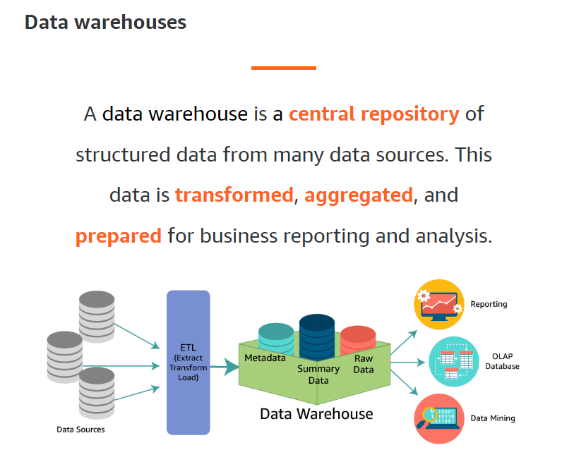
Data Processing Fundamentals
Data processing transforms raw data into meaningful information through systematic operations.
Processing Types
Batch Processing:
- Characteristics: Periodic processing of accumulated data
- Use Cases: Daily reports, ETL pipelines, historical analysis
- Advantages: Efficient for large volumes, predictable resource usage
- Tools: Apache Spark, AWS Glue, Apache Airflow
Stream Processing:
- Characteristics: Real-time processing of continuous data streams
- Use Cases: Fraud detection, real-time analytics, IoT monitoring
- Advantages: Low latency, immediate insights
- Tools: Apache Kafka, Apache Flink, AWS Kinesis
Real-Time Processing:
- Characteristics: Immediate processing with minimal delay
- Use Cases: Live dashboards, instant recommendations, alerts
- Advantages: Immediate action capability
- Tools: Apache Storm, AWS Lambda, Apache Kafka Streams
Data Structures and Storage
Relational Databases:
- Structured Query Language (SQL)
- ACID Transactions: Atomicity, Consistency, Isolation, Durability
- Normalized Schemas: Eliminating data redundancy
- Indexing: Optimizing query performance
NoSQL Databases:
- Document Stores: MongoDB, DynamoDB
- Key-Value Stores: Redis, DynamoDB
- Column-Family Stores: Cassandra, HBase
- Graph Databases: Neo4j, Amazon Neptune
Data Warehouses:
- Star Schema: Centralized fact tables with dimension tables
- Snowflake Schema: Normalized dimension tables
- Columnar Storage: Optimized for analytical queries
- MPP Architecture: Massively parallel processing
Varitey

Indexing

Data Integrity and Consistency
ACID Properties:
- Atomicity: All-or-nothing transaction execution
- Consistency: Database constraints and rules maintenance
- Isolation: Concurrent transaction independence
- Durability: Committed transaction persistence
BASE Properties:
- Basically Available: System remains operational despite failures
- Soft State: Temporary inconsistencies allowed
- Eventually Consistent: Convergence to consistent state over time
Choosing Between ACID and BASE:
# Example: Implementing consistency patterns
from boto3.dynamodb.conditions import Key, Attr
import boto3

def demonstrate_consistency_patterns():
    """Demonstrate different consistency approaches."""

    dynamodb = boto3.resource('dynamodb')
    table = dynamodb.Table('user-preferences')

    # Strongly consistent read (similar to ACID)
    def get_user_preferences_strong(user_id):
        """Get user preferences with strong consistency."""
        response = table.get_item(
            Key={'user_id': user_id},
            ConsistentRead=True  # Forces strong consistency
        )
        return response.get('Item')

    # Eventually consistent read (BASE approach)
    def get_user_preferences_eventual(user_id):
        """Get user preferences with eventual consistency."""
        response = table.get_item(
            Key={'user_id': user_id}
            # ConsistentRead=False is default - eventual consistency
        )
        return response.get('Item')

    # Conditional update (optimistic locking)
    def update_user_preferences_safe(user_id, preferences, expected_version):
        """Update with version check for consistency."""
        try:
            response = table.update_item(
                Key={'user_id': user_id},
                UpdateExpression="SET preferences = :prefs, version = version + :incr",
                ConditionExpression="version = :expected_version",
                ExpressionAttributeValues={
                    ':prefs': preferences,
                    ':incr': 1,
                    ':expected_version': expected_version
                },
                ReturnValues="ALL_NEW"
            )
            return {'success': True, 'item': response['Attributes']}
        except ClientError as e:
            if e.response['Error']['Code'] == 'ConditionalCheckFailedException':
                return {'success': False, 'error': 'Version conflict'}
            raise

    # Usage examples
    user_id = 'user123'

    # Strong consistency read
    prefs_strong = get_user_preferences_strong(user_id)

    # Eventual consistency read
    prefs_eventual = get_user_preferences_eventual(user_id)

    # Safe update
    update_result = update_user_preferences_safe(
        user_id,
        {'theme': 'dark', 'notifications': True},
        expected_version=5
    )

    return {
        'strong_consistency': prefs_strong,
        'eventual_consistency': prefs_eventual,
        'update_result': update_result
    }
Types of Data Analytics
Modern analytics encompasses various approaches, each serving different business needs.
Descriptive Analytics
What Happened?
- Purpose: Understanding historical data and current state
- Techniques: Data aggregation, reporting, dashboards
- Tools: Tableau, Power BI, Looker, custom SQL queries
Implementation Example:
# Descriptive analytics dashboard
import pandas as pd
import matplotlib.pyplot as plt
import seaborn as sns

def create_descriptive_dashboard(sales_data):
    """Create comprehensive descriptive analytics dashboard."""

    # Basic statistics
    summary_stats = sales_data.describe()

    # Time series analysis
    sales_data['order_date'] = pd.to_datetime(sales_data['order_date'])
    sales_data['month'] = sales_data['order_date'].dt.to_period('M')

    monthly_sales = sales_data.groupby('month')['amount'].agg([
        'sum', 'count', 'mean'
    ]).reset_index()

    # Customer segmentation
    customer_summary = sales_data.groupby('customer_id').agg({
        'amount': ['sum', 'count', 'mean'],
        'order_date': ['min', 'max']
    }).reset_index()

    customer_summary.columns = ['customer_id', 'total_spent', 'order_count',
                               'avg_order_value', 'first_order', 'last_order']

    # Product performance
    product_performance = sales_data.groupby('product_category').agg({
        'amount': 'sum',
        'order_id': 'count'
    }).sort_values('amount', ascending=False)

    # Create visualizations
    fig, axes = plt.subplots(2, 2, figsize=(15, 10))

    # Monthly sales trend
    monthly_sales['month'] = monthly_sales['month'].astype(str)
    axes[0, 0].plot(monthly_sales['month'], monthly_sales['sum'])
    axes[0, 0].set_title('Monthly Sales Trend')
    axes[0, 0].tick_params(axis='x', rotation=45)

    # Customer distribution
    axes[0, 1].hist(customer_summary['total_spent'], bins=50, alpha=0.7)
    axes[0, 1].set_title('Customer Spending Distribution')
    axes[0, 1].set_xlabel('Total Spent')
    axes[0, 1].set_ylabel('Number of Customers')

    # Top product categories
    top_categories = product_performance.head(10)
    axes[1, 0].bar(range(len(top_categories)), top_categories['amount'])
    axes[1, 0].set_xticks(range(len(top_categories)))
    axes[1, 0].set_xticklabels(top_categories.index, rotation=45)
    axes[1, 0].set_title('Top Product Categories by Revenue')

    # Order value distribution
    axes[1, 1].boxplot(sales_data['amount'])
    axes[1, 1].set_title('Order Value Distribution')

    plt.tight_layout()
    plt.show()

    return {
        'summary_stats': summary_stats,
        'monthly_sales': monthly_sales,
        'customer_summary': customer_summary,
        'product_performance': product_performance
    }

# Generate dashboard
dashboard_data = create_descriptive_dashboard(sales_df)
Diagnostic Analytics
Why Did It Happen?
- Purpose: Identifying root causes and underlying factors
- Techniques: Drill-down analysis, correlation analysis, hypothesis testing
- Tools: Statistical software, A/B testing platforms, regression analysis
Root Cause Analysis:
# Diagnostic analytics: Root cause analysis
from scipy import stats
import statsmodels.api as sm
from statsmodels.formula.api import ols

def perform_root_cause_analysis(sales_data, external_factors):
    """Perform diagnostic analysis to identify sales drivers."""

    # Correlation analysis
    correlation_matrix = sales_data.corr()

    # Key correlations with sales
    sales_correlations = correlation_matrix['sales_amount'].sort_values(ascending=False)

    # Regression analysis
    # Prepare features
    features = ['marketing_spend', 'season', 'competitor_price', 'economic_indicator']
    X = sales_data[features]
    y = sales_data['sales_amount']

    # Add constant for intercept
    X = sm.add_constant(X)

    # Fit regression model
    model = sm.OLS(y, X).fit()

    # Regression results
    regression_summary = model.summary()

    # ANOVA for categorical factors
    anova_model = ols('sales_amount ~ C(season) + C(region)', data=sales_data).fit()
    anova_table = sm.stats.anova_lm(anova_model, typ=2)

    # External factor impact analysis
    external_impact = {}
    for factor in external_factors:
        correlation = stats.pearsonr(sales_data['sales_amount'],
                                   external_factors[factor])[0]
        external_impact[factor] = correlation

    # Identify key drivers
    key_drivers = {
        'top_correlations': sales_correlations.head(5),
        'regression_coefficients': model.params,
        'significant_factors': model.pvalues[model.pvalues < 0.05],
        'anova_results': anova_table,
        'external_factors_impact': external_impact
    }

    return key_drivers

# Example usage
external_factors = {
    'weather_index': sales_df['weather_score'],
    'holiday_flag': sales_df['is_holiday'],
    'economic_index': sales_df['economic_indicator']
}

diagnostic_results = perform_root_cause_analysis(sales_df, external_factors)
print("Key Sales Drivers Identified:")
print(diagnostic_results['top_correlations'])
Predictive Analytics
What Will Happen?
- Purpose: Forecasting future outcomes and trends
- Techniques: Machine learning models, time series analysis, statistical forecasting
- Tools: Scikit-learn, TensorFlow, Prophet, ARIMA models
Time Series Forecasting:
# Predictive analytics: Time series forecasting
from prophet import Prophet
import pandas as pd
from sklearn.metrics import mean_absolute_error, mean_squared_error

def forecast_sales_prophet(historical_data, forecast_periods=30):
    """Forecast future sales using Facebook Prophet."""

    # Prepare data for Prophet
    prophet_data = historical_data[['order_date', 'amount']].copy()
    prophet_data.columns = ['ds', 'y']  # Prophet requires 'ds' and 'y' columns

    # Initialize and fit model
    model = Prophet(
        yearly_seasonality=True,
        weekly_seasonality=True,
        daily_seasonality=False,
        seasonality_mode='multiplicative'
    )

    # Add holidays if available
    if 'is_holiday' in historical_data.columns:
        holidays = historical_data[historical_data['is_holiday'] == 1][['order_date']]
        holidays.columns = ['ds']
        holidays['holiday'] = 'holiday'
        model.add_country_holidays(country_name='US')

    model.fit(prophet_data)

    # Create future dataframe
    future = model.make_future_dataframe(periods=forecast_periods)

    # Generate forecast
    forecast = model.predict(future)

    # Extract forecast components
    forecast_components = {
        'trend': forecast[['ds', 'trend']],
        'seasonal': forecast[['ds', 'yearly', 'weekly']],
        'forecast': forecast[['ds', 'yhat', 'yhat_lower', 'yhat_upper']]
    }

    # Model evaluation (if we have actual future data)
    if len(historical_data) > forecast_periods:
        # Split data for validation
        train_size = len(historical_data) - forecast_periods
        train_data = prophet_data[:train_size]
        test_data = prophet_data[train_size:]

        # Refit on training data
        eval_model = Prophet(yearly_seasonality=True, weekly_seasonality=True)
        eval_model.fit(train_data)

        # Forecast on test period
        future_eval = eval_model.make_future_dataframe(periods=forecast_periods)
        forecast_eval = eval_model.predict(future_eval)

        # Calculate metrics
        mae = mean_absolute_error(test_data['y'], forecast_eval['yhat'][-forecast_periods:])
        rmse = np.sqrt(mean_squared_error(test_data['y'], forecast_eval['yhat'][-forecast_periods:]))

        evaluation_metrics = {
            'mae': mae,
            'rmse': rmse,
            'mape': np.mean(np.abs((test_data['y'] - forecast_eval['yhat'][-forecast_periods:]) / test_data['y'])) * 100
        }
    else:
        evaluation_metrics = None

    return {
        'model': model,
        'forecast': forecast_components,
        'evaluation': evaluation_metrics
    }

# Generate sales forecast
forecast_results = forecast_sales_prophet(sales_df, forecast_periods=90)

# Plot forecast
model = forecast_results['model']
forecast_plot = model.plot(forecast_results['forecast']['forecast'])
plt.title('Sales Forecast with Prophet')
plt.show()

if forecast_results['evaluation']:
    print(f"Forecast Accuracy - MAE: ${forecast_results['evaluation']['mae']:.2f}")
    print(f"Forecast Accuracy - RMSE: ${forecast_results['evaluation']['rmse']:.2f}")
Prescriptive Analytics
What Should We Do?
- Purpose: Recommending optimal actions and decisions
- Techniques: Optimization algorithms, simulation, decision trees
- Tools: Linear programming solvers, simulation software, reinforcement learning
Optimization Example:
# Prescriptive analytics: Resource optimization
from scipy.optimize import linprog
import numpy as np

def optimize_inventory_allocation(demand_forecast, current_inventory, constraints):
    """
    Optimize inventory allocation across regions using linear programming.
    """

    # Objective: Minimize total cost (holding + shortage costs)
    # Subject to: Supply constraints, demand satisfaction

    n_regions = len(demand_forecast)
    n_products = len(demand_forecast[0])

    # Flatten decision variables: allocation[region][product]
    n_variables = n_regions * n_products

    # Cost coefficients (holding costs per unit)
    holding_costs = constraints['holding_costs']  # [product][region]
    c = holding_costs.flatten()

    # Constraint 1: Total allocation per product <= available inventory
    A_ub = []
    b_ub = []

    for product in range(n_products):
        constraint_row = []
        for region in range(n_regions):
            for p in range(n_products):
                if p == product:
                    constraint_row.append(1)
                else:
                    constraint_row.append(0)
        A_ub.append(constraint_row)
        b_ub.append(current_inventory[product])

    A_ub = np.array(A_ub)
    b_ub = np.array(b_ub)

    # Constraint 2: Allocation per region/product >= 0 (handled by bounds)
    # Constraint 3: Meet minimum demand satisfaction
    for region in range(n_regions):
        for product in range(n_products):
            constraint_row = []
            for r in range(n_regions):
                for p in range(n_products):
                    if r == region and p == product:
                        constraint_row.append(-1)  # -allocation >= -demand
                    else:
                        constraint_row.append(0)
            A_ub = np.vstack([A_ub, constraint_row])
            b_ub = np.append(b_ub, -demand_forecast[region][product] * constraints['min_service_level'])

    # Bounds: allocation >= 0
    bounds = [(0, None) for _ in range(n_variables)]

    # Solve optimization
    result = linprog(c, A_ub=A_ub, b_ub=b_ub, bounds=bounds, method='highs')

    if result.success:
        # Reshape solution
        allocation = result.x.reshape((n_regions, n_products))

        # Calculate total cost
        total_cost = np.sum(allocation * holding_costs)

        # Calculate service levels
        service_levels = np.minimum(allocation / demand_forecast, 1) * 100

        return {
            'success': True,
            'allocation': allocation,
            'total_cost': total_cost,
            'service_levels': service_levels,
            'cost_breakdown': allocation * holding_costs
        }
    else:
        return {
            'success': False,
            'message': result.message
        }

# Example optimization
demand_forecast = np.array([
    [100, 150, 80],  # Region 1 demand for products A, B, C
    [120, 130, 90],  # Region 2
    [90, 140, 110]   # Region 3
])

current_inventory = np.array([280, 350, 250])  # Available inventory per product

constraints = {
    'holding_costs': np.array([
        [2.5, 3.0, 2.8],  # Product A holding costs by region
        [3.2, 2.7, 3.5],  # Product B
        [2.9, 3.1, 2.6]   # Product C
    ]),
    'min_service_level': 0.95  # 95% minimum service level
}

optimization_result = optimize_inventory_allocation(
    demand_forecast, current_inventory, constraints
)

if optimization_result['success']:
    print("Optimal Inventory Allocation:")
    print(optimization_result['allocation'])
    print(f"Total Cost: ${optimization_result['total_cost']:.2f}")
    print("Service Levels (%):")
    print(optimization_result['service_levels'])
Conclusion: Building Analytics Excellence
Data analytics fundamentals provide the foundation for transforming raw data into actionable knowledge that drives business decisions, operational improvements, and strategic planning. By understanding the core concepts, methodologies, and technologies covered in this guide, organizations can build robust analytics capabilities that deliver competitive advantage.
Key principles for analytics success include:
- Data Quality First: Ensuring clean, reliable data as the foundation
- Scalable Architecture: Building systems that grow with data needs
- Governance and Security: Protecting data while enabling access
- Continuous Learning: Evolving analytics capabilities with business needs
- Business Alignment: Focusing analytics efforts on strategic objectives
The journey from data to insights requires both technical expertise and business acumen. By following systematic approaches and leveraging modern tools and platforms, organizations can unlock the full potential of their data assets.
Comprehensive guide to data analytics fundamentals, covering core concepts, methodologies, and practical implementation strategies.