Machine Learning Pipeline on AWS

January 29, 2025

Building End-to-End Machine Learning Pipelines on AWS

Machine learning pipelines represent the systematic approach to transforming raw data into production-ready models that deliver business value. This comprehensive guide explores the complete ML pipeline lifecycle on AWS, from problem formulation to model deployment, with practical examples and best practices for building scalable, reliable ML solutions.

The ML Pipeline Lifecycle: A Comprehensive Overview

A machine learning pipeline is a systematic workflow that transforms raw data into actionable insights through a series of interconnected stages. Each stage builds upon the previous one, creating a robust framework for developing, deploying, and maintaining ML models in production environments.

Core Pipeline Components

Data + Algorithm + Compute = Model

The fundamental equation of machine learning combines three essential elements:

Data: The fuel that powers ML models
Algorithm: The mathematical approach to learning patterns
Compute: The infrastructure resources for training and inference

Business Problem Translation

Consider a common e-commerce scenario: predicting customer purchase likelihood based on browsing behavior. This business need translates into a technical ML problem through systematic decomposition.

Business Requirements:

Predict purchase probability for website visitors
Enable personalized marketing campaigns
Optimize product recommendations
Improve conversion rates

Technical Translation:

Binary classification problem (purchase/no-purchase)
Features: browsing time, pages viewed, cart additions, search terms
Target metric: prediction accuracy > 85%
Business impact: 15% increase in conversion rate

Classical Programming vs. Machine Learning Paradigms

Understanding the fundamental difference between traditional programming and ML is crucial for effective pipeline design.

Traditional Programming Approach

Input + Rules = Output

Rules: Explicitly defined by developers
Logic: Deterministic and predictable
Maintenance: Manual updates required
Scalability: Limited by rule complexity

Machine Learning Approach

Input + Output = Rules (Model)

Rules: Automatically learned from data
Logic: Probabilistic and adaptive
Maintenance: Self-improving through new data
Scalability: Improves with more data and compute

Learning Paradigms: Choosing the Right Approach

Supervised Learning: Labeled Data-Driven Models

Supervised learning forms the backbone of most business ML applications, using labeled examples to train predictive models.

Core Characteristics:

Training data includes both input features and correct outputs
Model learns mapping between inputs and desired outputs
Performance measured against known correct answers

Types of Supervised Learning:

Binary Classification:

Predicts one of two possible outcomes
Examples: Spam detection, fraud identification, customer churn prediction
Evaluation metrics: Accuracy, Precision, Recall, F1-Score, AUC-ROC

Multiclass Classification:

Predicts one of multiple categorical outcomes
Examples: Product categorization, sentiment analysis, image classification
Evaluation metrics: Accuracy, macro/micro F1, confusion matrix

Regression:

Predicts continuous numerical values
Examples: Price prediction, demand forecasting, risk scoring
Evaluation metrics: MSE, RMSE, MAE, R²

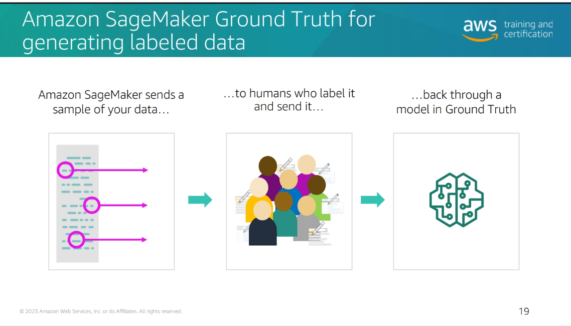
Amazon SageMaker Ground Truth for Labeling:

import boto3

# Create a labeling job
sagemaker = boto3.client('sagemaker')

response = sagemaker.create_labeling_job(
    LabelingJobName='customer-churn-labeling',
    LabelAttributeName='churn-label',
    InputConfig={
        'DataSource': {
            'S3DataSource': {
                'ManifestS3Uri': 's3://my-bucket/input.manifest'
            }
        }
    },
    OutputConfig={
        'S3OutputPath': 's3://my-bucket/output/'
    },
    RoleArn='arn:aws:iam::123456789012:role/SageMakerRole',
    HumanTaskConfig={
        'WorkteamArn': 'arn:aws:sagemaker:us-east-1:123456789012:workteam/private-crowd/my-workteam',
        'UiConfig': {
            'UiTemplateS3Uri': 's3://my-bucket/ui-template.html'
        },
        'TaskTitle': 'Classify customer churn risk',
        'TaskDescription': 'Determine if customer is likely to churn',
        'NumberOfHumanWorkersPerDataObject': 3,
        'TaskTimeLimitInSeconds': 300,
        'TaskAvailabilityLifetimeInSeconds': 864000
    }
)

Unsupervised Learning: Pattern Discovery

Unsupervised learning uncovers hidden structures in data without labeled examples.

Key Applications:

Customer segmentation and clustering
Anomaly detection
Dimensionality reduction
Topic modeling

Popular Algorithms:

K-Means clustering
Principal Component Analysis (PCA)
Autoencoders
Gaussian Mixture Models

Reinforcement Learning: Decision-Making Systems

Reinforcement learning trains agents to make sequential decisions through trial-and-error.

Core Components:

Agent: Decision-making entity
Environment: System the agent interacts with
Actions: Possible decisions the agent can make
Rewards: Feedback signals for good/bad decisions
Policy: Strategy for choosing actions

Applications:

Game playing (AlphaGo, Dota 2)
Robotics and autonomous systems
Recommendation systems
Resource optimization

Deep Learning: Neural Network Revolution

Deep learning represents a subset of machine learning that uses artificial neural networks with multiple layers to learn complex patterns.

Neural Network Architecture

Basic Neuron Structure:

Input → Weights → Activation Function → Output

Deep Network Characteristics:

Multiple hidden layers between input and output
Non-linear activation functions (ReLU, sigmoid, tanh)
Backpropagation for weight optimization
Gradient descent for parameter updates

Deep Learning Advantages

Feature Learning:

Automatically extracts hierarchical features
No manual feature engineering required
Learns from raw data (images, text, audio)

Scalability:

Performance improves with more data
Parallel processing on GPUs/TPUs
Handles high-dimensional data effectively

Popular Deep Learning Frameworks

TensorFlow:

import tensorflow as tf

# Define a simple neural network
model = tf.keras.Sequential([
    tf.keras.layers.Dense(128, activation='relu', input_shape=(784,)),
    tf.keras.layers.Dropout(0.2),
    tf.keras.layers.Dense(10, activation='softmax')
])

# Compile and train
model.compile(optimizer='adam',
              loss='sparse_categorical_crossentropy',
              metrics=['accuracy'])

model.fit(x_train, y_train, epochs=5)

PyTorch:

import torch
import torch.nn as nn

class SimpleNN(nn.Module):
    def __init__(self):
        super(SimpleNN, self).__init__()
        self.fc1 = nn.Linear(784, 128)
        self.fc2 = nn.Linear(128, 10)
        self.dropout = nn.Dropout(0.2)

    def forward(self, x):
        x = torch.relu(self.fc1(x))
        x = self.dropout(x)
        x = self.fc2(x)
        return x

model = SimpleNN()
criterion = nn.CrossEntropyLoss()
optimizer = torch.optim.Adam(model.parameters())

ML Pipeline Stages: From Concept to Production

Stage 1: Problem Formulation

Business Problem Definition:

What business outcome are we trying to achieve?
What is the measurable impact of success?
What are the constraints and requirements?

Technical Problem Translation:

What type of ML problem is this?
What data do we need?
What performance metrics matter?

Success Criteria Definition:

Model Performance Metrics:

Accuracy: Overall correctness of predictions
Precision: True positives / (True positives + False positives)
Recall: True positives / (True positives + False negatives)
F1-Score: Harmonic mean of precision and recall
AUC-ROC: Area under the receiver operating characteristic curve

Business Impact Metrics:

Revenue increase from better predictions
Cost reduction from optimized operations
Customer satisfaction improvements
Operational efficiency gains

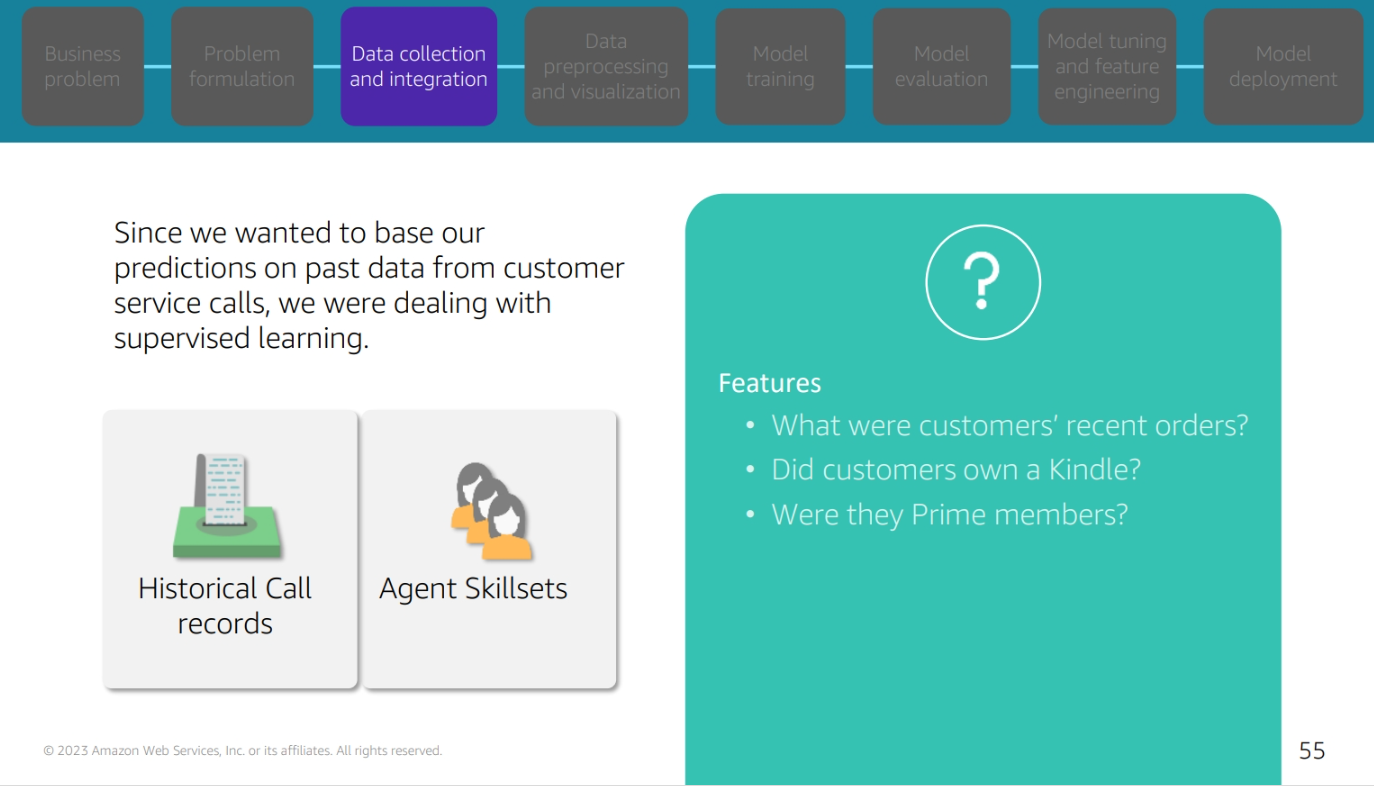
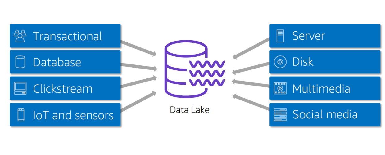
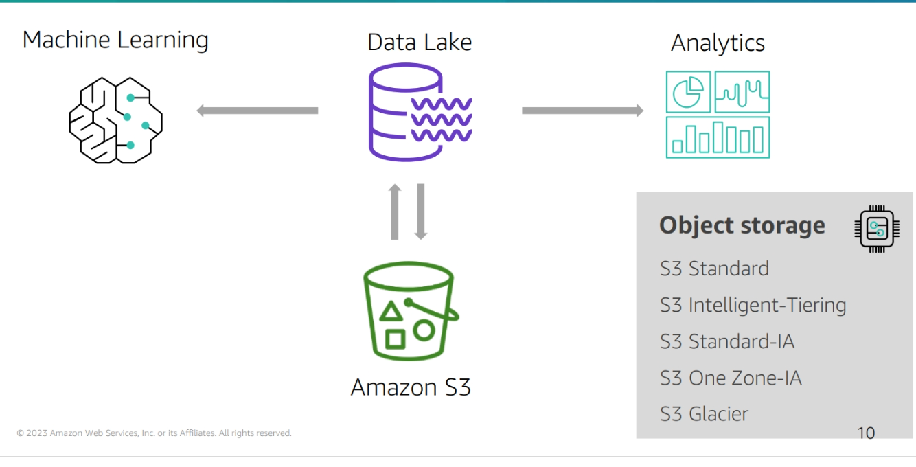
Stage 2: Data Collection and Integration

Data Sources:

Internal databases and data warehouses
External APIs and third-party data
Streaming data from IoT devices
User-generated content and logs

AWS Data Ingestion Services:

Amazon S3 for Data Lake:

import boto3

# Upload data to S3
s3 = boto3.client('s3')
s3.upload_file('local_data.csv', 'my-data-lake', 'raw/customer_data.csv')

AWS Glue for ETL:

import boto3
from pyspark.sql import SparkSession

glue = boto3.client('glue')

# Create ETL job
response = glue.create_job(
    Name='customer-data-etl',
    Role='arn:aws:iam::123456789012:role/GlueRole',
    Command={
        'Name': 'glueetl',
        'ScriptLocation': 's3://my-scripts/etl_script.py'
    },
    DefaultArguments={
        '--job-bookmark-option': 'job-bookmark-enable'
    }
)

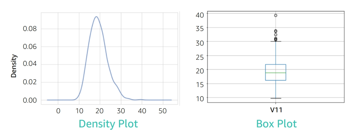
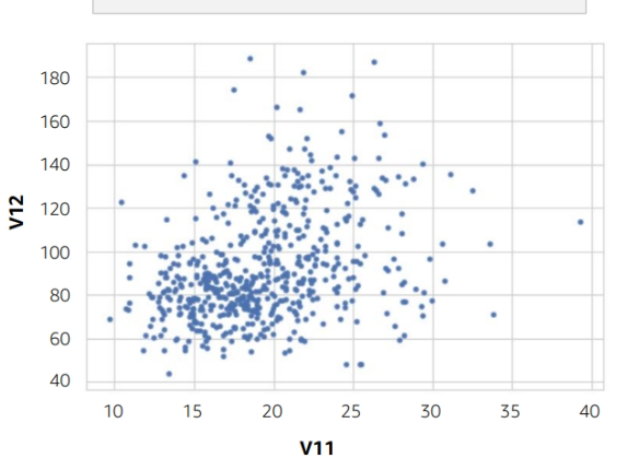
Stage 3: Data Preprocessing and Exploration

Data Quality Assessment:

Missing value analysis
Outlier detection
Data type validation
Statistical distribution checks

Essential Python Libraries:

Pandas for Data Manipulation:

import pandas as pd

# Load and explore data
df = pd.read_csv('customer_data.csv')

# Basic exploration
print(df.head())
print(df.describe())
print(df.isnull().sum())

# Handle missing values
df['age'].fillna(df['age'].median(), inplace=True)
df['income'].fillna(df['income'].mean(), inplace=True)

NumPy for Numerical Operations:

import numpy as np

# Array operations
data = np.array([[1, 2, 3], [4, 5, 6]])
normalized = (data - np.min(data)) / (np.max(data) - np.min(data))

Data Visualization:

import matplotlib.pyplot as plt
import seaborn as sns

# Distribution plots
plt.figure(figsize=(10, 6))
sns.histplot(df['age'], bins=30)
plt.title('Age Distribution')
plt.show()

# Correlation heatmap
plt.figure(figsize=(12, 8))
sns.heatmap(df.corr(), annot=True, cmap='coolwarm')
plt.title('Feature Correlations')
plt.show()

Outlier Detection Techniques:

Statistical Methods:

# Z-score method
from scipy import stats

z_scores = stats.zscore(df['income'])
outliers = df[abs(z_scores) > 3]

# IQR method
Q1 = df['income'].quantile(0.25)
Q3 = df['income'].quantile(0.75)
IQR = Q3 - Q1
outliers = df[(df['income'] < Q1 - 1.5 * IQR) | (df['income'] > Q3 + 1.5 * IQR)]

Machine Learning Methods:

from sklearn.ensemble import IsolationForest

# Isolation Forest for outlier detection
iso_forest = IsolationForest(contamination=0.1, random_state=42)
outliers = iso_forest.fit_predict(df[['age', 'income']])
outlier_data = df[outliers == -1]

Stage 4: Feature Engineering

Feature Selection:

Remove irrelevant or redundant features
Identify most predictive variables
Reduce dimensionality and computational cost

Feature Extraction:

Create new features from existing data
Domain knowledge application
Automated feature generation

Feature Transformation:

Normalization and scaling
Encoding categorical variables
Handling skewed distributions

Scaling Techniques:

Min-Max Scaling:

from sklearn.preprocessing import MinMaxScaler

scaler = MinMaxScaler()
scaled_features = scaler.fit_transform(df[['age', 'income']])

Standardization:

from sklearn.preprocessing import StandardScaler

scaler = StandardScaler()
standardized_features = scaler.fit_transform(df[['age', 'income']])

Categorical Encoding:

One-Hot Encoding:

from sklearn.preprocessing import OneHotEncoder

encoder = OneHotEncoder(sparse=False)
encoded_features = encoder.fit_transform(df[['category']])

Label Encoding:

from sklearn.preprocessing import LabelEncoder

encoder = LabelEncoder()
encoded_labels = encoder.fit_transform(df['target'])

Stage 5: Model Training and Evaluation

Model Selection Framework:

Start with simple models (baseline)
Progress to complex models
Compare performance across algorithms
Consider computational constraints

Training Best Practices:

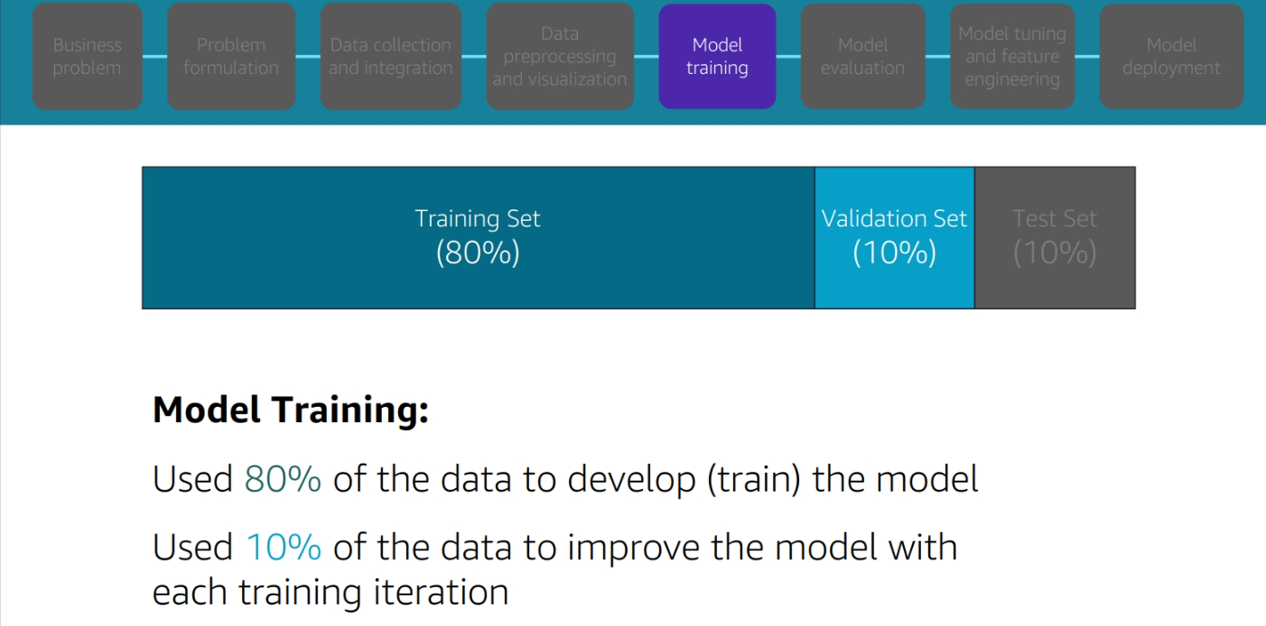
Data Splitting:

from sklearn.model_selection import train_test_split

X_train, X_test, y_train, y_test = train_test_split(
    X, y, test_size=0.2, random_state=42, stratify=y
)

X_train, X_val, y_train, y_val = train_test_split(
    X_train, y_train, test_size=0.2, random_state=42, stratify=y_train
)

Cross-Validation:

from sklearn.model_selection import cross_val_score
from sklearn.ensemble import RandomForestClassifier

model = RandomForestClassifier(random_state=42)
scores = cross_val_score(model, X_train, y_train, cv=5, scoring='accuracy')
print(f"Cross-validation accuracy: {scores.mean():.3f} (+/- {scores.std() * 2:.3f})")

Overfitting vs. Underfitting:

Bias-Variance Tradeoff:

High Bias (Underfitting): Model too simple, misses patterns
High Variance (Overfitting): Model too complex, memorizes noise
Balanced Model: Optimal complexity for generalization

Regularization Techniques:

from sklearn.linear_model import LogisticRegression

# L1 regularization (Lasso)
model_l1 = LogisticRegression(penalty='l1', C=0.1, solver='liblinear')

# L2 regularization (Ridge)
model_l2 = LogisticRegression(penalty='l2', C=0.1)

# Elastic Net (combination)
model_en = LogisticRegression(penalty='elasticnet', C=0.1, l1_ratio=0.5, solver='saga')

Evaluation Metrics Deep Dive:

Confusion Matrix Analysis:

from sklearn.metrics import confusion_matrix, classification_report

y_pred = model.predict(X_test)
cm = confusion_matrix(y_test, y_pred)

print("Confusion Matrix:")
print(cm)
print("\nClassification Report:")
print(classification_report(y_test, y_pred))

ROC Curve and AUC:

from sklearn.metrics import roc_curve, auc
import matplotlib.pyplot as plt

# Get prediction probabilities
y_prob = model.predict_proba(X_test)[:, 1]

# Calculate ROC curve
fpr, tpr, thresholds = roc_curve(y_test, y_prob)
roc_auc = auc(fpr, tpr)

# Plot ROC curve
plt.figure(figsize=(8, 6))
plt.plot(fpr, tpr, color='darkorange', lw=2, label=f'ROC curve (AUC = {roc_auc:.2f})')
plt.plot([0, 1], [0, 1], color='navy', lw=2, linestyle='--')
plt.xlabel('False Positive Rate')
plt.ylabel('True Positive Rate')
plt.title('Receiver Operating Characteristic (ROC) Curve')
plt.legend(loc="lower right")
plt.show()

Stage 6: Hyperparameter Tuning

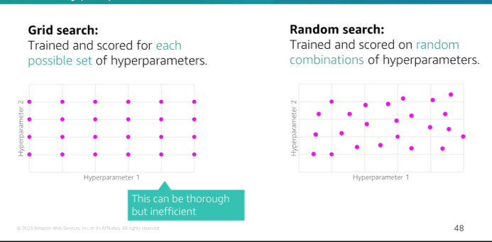
Grid Search:

from sklearn.model_selection import GridSearchCV

param_grid = {
    'n_estimators': [100, 200, 300],
    'max_depth': [10, 20, None],
    'min_samples_split': [2, 5, 10]
}

grid_search = GridSearchCV(
    RandomForestClassifier(random_state=42),
    param_grid,
    cv=5,
    scoring='accuracy',
    n_jobs=-1
)

grid_search.fit(X_train, y_train)
print(f"Best parameters: {grid_search.best_params_}")
print(f"Best cross-validation score: {grid_search.best_score_:.3f}")

Random Search:

from sklearn.model_selection import RandomizedSearchCV
from scipy.stats import randint

param_dist = {
    'n_estimators': randint(100, 500),
    'max_depth': [10, 20, 30, None],
    'min_samples_split': randint(2, 20)
}

random_search = RandomizedSearchCV(
    RandomForestClassifier(random_state=42),
    param_dist,
    n_iter=50,
    cv=5,
    scoring='accuracy',
    n_jobs=-1,
    random_state=42
)

random_search.fit(X_train, y_train)

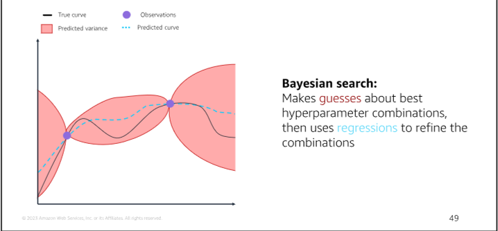
Bayesian Optimization:

from skopt import BayesSearchCV

param_space = {
    'n_estimators': (100, 500),
    'max_depth': (10, 50),
    'min_samples_split': (2, 20)
}

bayes_search = BayesSearchCV(
    RandomForestClassifier(random_state=42),
    param_space,
    n_iter=50,
    cv=5,
    scoring='accuracy',
    n_jobs=-1,
    random_state=42
)

bayes_search.fit(X_train, y_train)

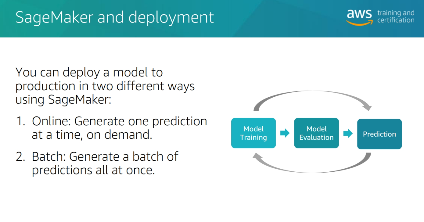
Stage 7: Model Deployment and Serving

Deployment Strategies:

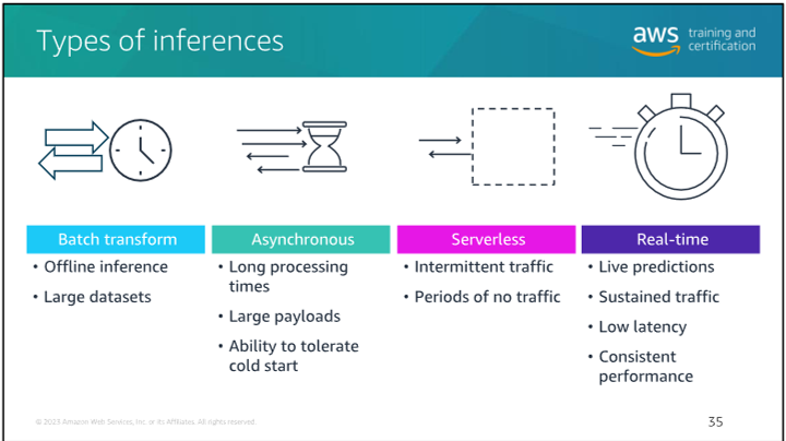
Batch Inference:

Process large datasets periodically
Cost-effective for non-real-time use cases
Suitable for daily/weekly predictions

Real-time Inference:

Low-latency predictions for immediate responses
Required for user-facing applications
Higher infrastructure costs

AWS SageMaker Deployment:

Model Creation:

import boto3
from sagemaker import get_execution_role
from sagemaker.model import Model

role = get_execution_role()
sagemaker_client = boto3.client('sagemaker')

# Create SageMaker model
model = Model(
    model_data='s3://my-bucket/models/model.tar.gz',
    image_uri='683313688378.dkr.ecr.us-east-1.amazonaws.com/sagemaker-scikit-learn:0.23-1-cpu-py3',
    role=role,
    sagemaker_session=sagemaker_session
)

Endpoint Deployment:

# Deploy to endpoint
predictor = model.deploy(
    initial_instance_count=1,
    instance_type='ml.m5.large',
    endpoint_name='customer-churn-endpoint'
)

# Make predictions
predictions = predictor.predict(test_data)

Blue-Green Deployment:

# Create new endpoint with updated model
new_model = Model(
    model_data='s3://my-bucket/models/new-model.tar.gz',
    image_uri='683313688378.dkr.ecr.us-east-1.amazonaws.com/sagemaker-scikit-learn:0.23-1-cpu-py3',
    role=role
)

new_predictor = new_model.deploy(
    initial_instance_count=1,
    instance_type='ml.m5.large',
    endpoint_name='customer-churn-endpoint-v2'
)

# Test new endpoint
# If successful, update production traffic
# Delete old endpoint

Canary Deployment:

# Deploy canary endpoint
canary_predictor = new_model.deploy(
    initial_instance_count=1,
    instance_type='ml.m5.large',
    endpoint_name='customer-churn-canary'
)

# Route 10% of traffic to canary
# Monitor performance metrics
# Gradually increase traffic if successful

Monitoring and Maintenance

Model Performance Monitoring:

Prediction accuracy drift
Data distribution changes
Latency and throughput metrics
Error rate analysis

Automated Retraining:

# SageMaker Pipelines for automated retraining
from sagemaker.workflow.pipeline import Pipeline
from sagemaker.workflow.steps import TrainingStep, ProcessingStep

# Define steps for automated retraining pipeline
# Trigger based on performance degradation or schedule

Best Practices for Production ML Pipelines

1. Data Management

Implement data versioning and lineage tracking
Establish data quality monitoring
Create reproducible data pipelines
Maintain data privacy and security

2. Model Development

Use experiment tracking (MLflow, SageMaker Experiments)
Implement proper validation procedures
Document model assumptions and limitations
Establish model review and approval processes

3. Deployment and Operations

Implement gradual rollout strategies
Set up comprehensive monitoring
Create rollback procedures
Establish incident response protocols

4. Governance and Compliance

Maintain model audit trails
Implement access controls
Ensure regulatory compliance
Document model decisions and limitations

Future Trends in ML Pipelines

AutoML and Meta-Learning

Automated model selection and hyperparameter tuning
Neural architecture search
Meta-learning for few-shot learning

Edge ML and Federated Learning

Model deployment on edge devices
Privacy-preserving distributed learning
Real-time adaptation to local conditions

MLOps 2.0

AI-assisted pipeline optimization
Automated model lifecycle management
Continuous learning systems
Ethical AI and bias mitigation

Conclusion: Building Robust ML Pipelines

Successful machine learning pipelines require careful attention to each stage of the process, from problem formulation to production deployment. AWS provides comprehensive tools and services to support every aspect of the ML lifecycle, enabling organizations to build scalable, reliable, and maintainable ML solutions.

Key success factors include:

Strong Foundation: Clear problem definition and success metrics
Quality Data: Comprehensive data collection and preprocessing
Rigorous Evaluation: Thorough model validation and testing
Production Readiness: Robust deployment and monitoring
Continuous Improvement: Ongoing optimization and maintenance

By following these principles and leveraging AWS's powerful ML services, organizations can transform their data into actionable insights that drive real business value.

Comprehensive guide to building end-to-end machine learning pipelines on AWS, covering the complete ML lifecycle from problem formulation to production deployment.

Deep Learning

Deep Learning:
- A type of machine learning
- Uses neural networks
- Can learn from unstructured data
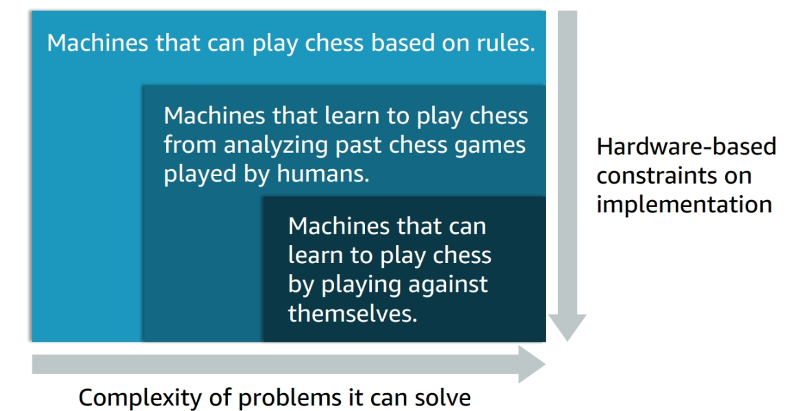
The figure demonstate going from AI to ML to Deep Learning

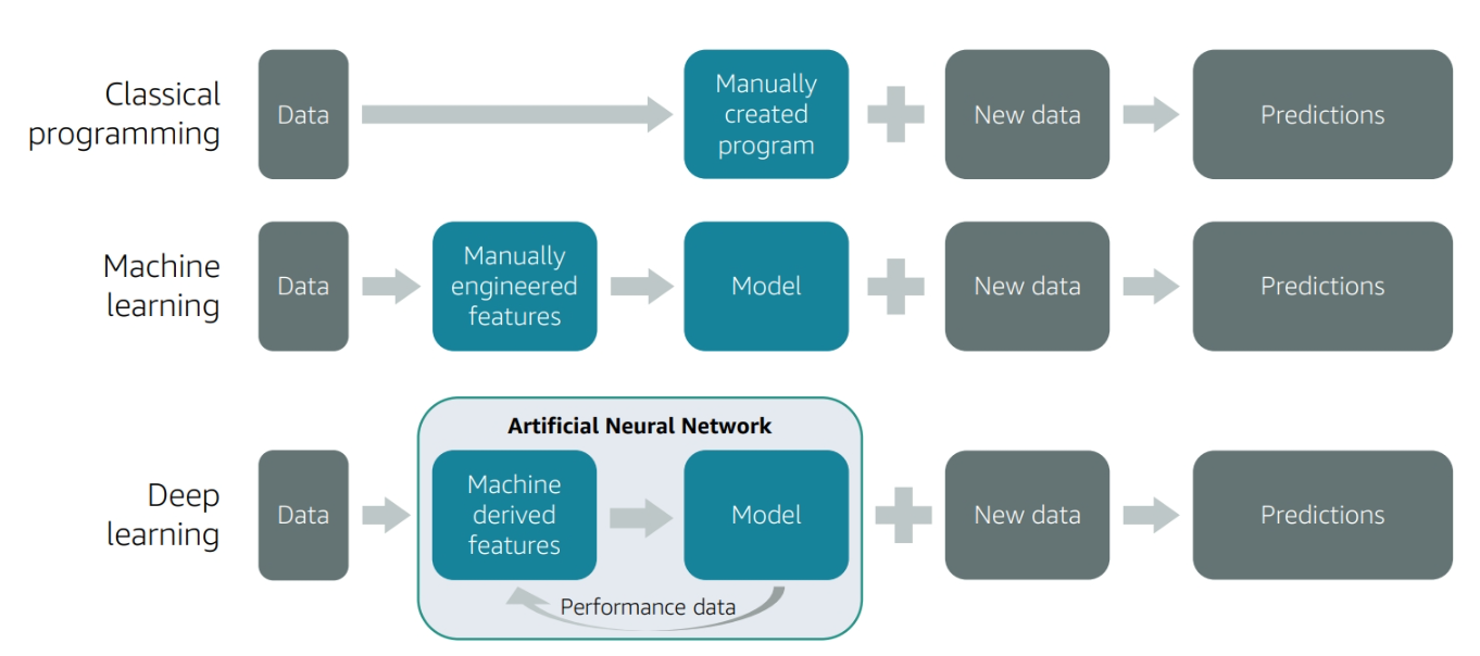
Deep Learning recap

Deep learning models
- Learn using Artificial Neural Networks (ANN)
- Can be trained on raw features
Include:
- A subset of ML methods
- Neurons arranged for computational efficiency
- Training networks with hundreds of layers that learn and improve the features

Machine Learning use cases

Recommendation Systems: Predicting what a user will like
Fraud Detection: Predicting whether a transaction is fraudulent
Voice Recognition: Predicting what a user is saying.
Image Recognition: Predicting what is in an image

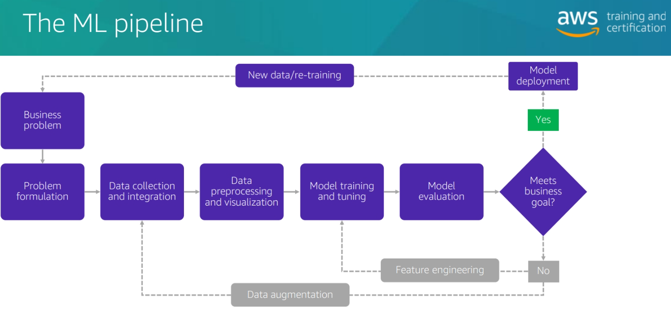
The Pipeline of ML Problem for buy kindle

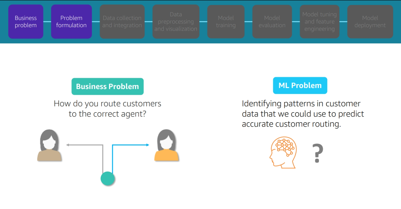
Bussines problem and Problem Formulation

Data collection and integration

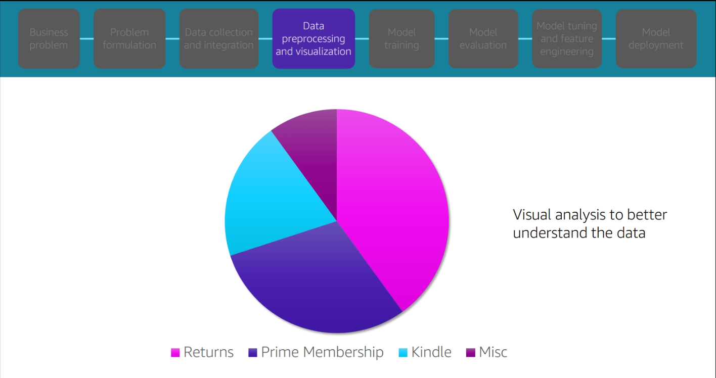
Data preprocessing and visulization

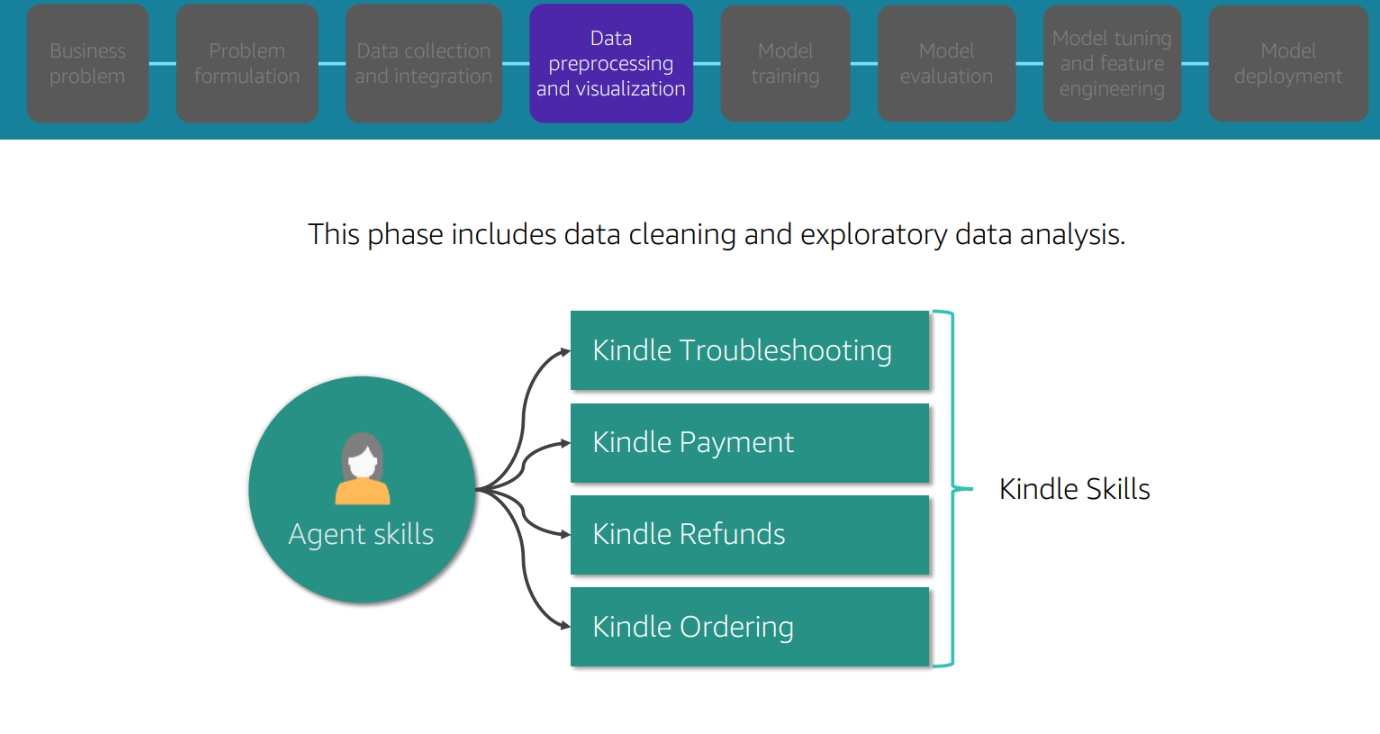
Data prepprocessing and visualization

Model Training

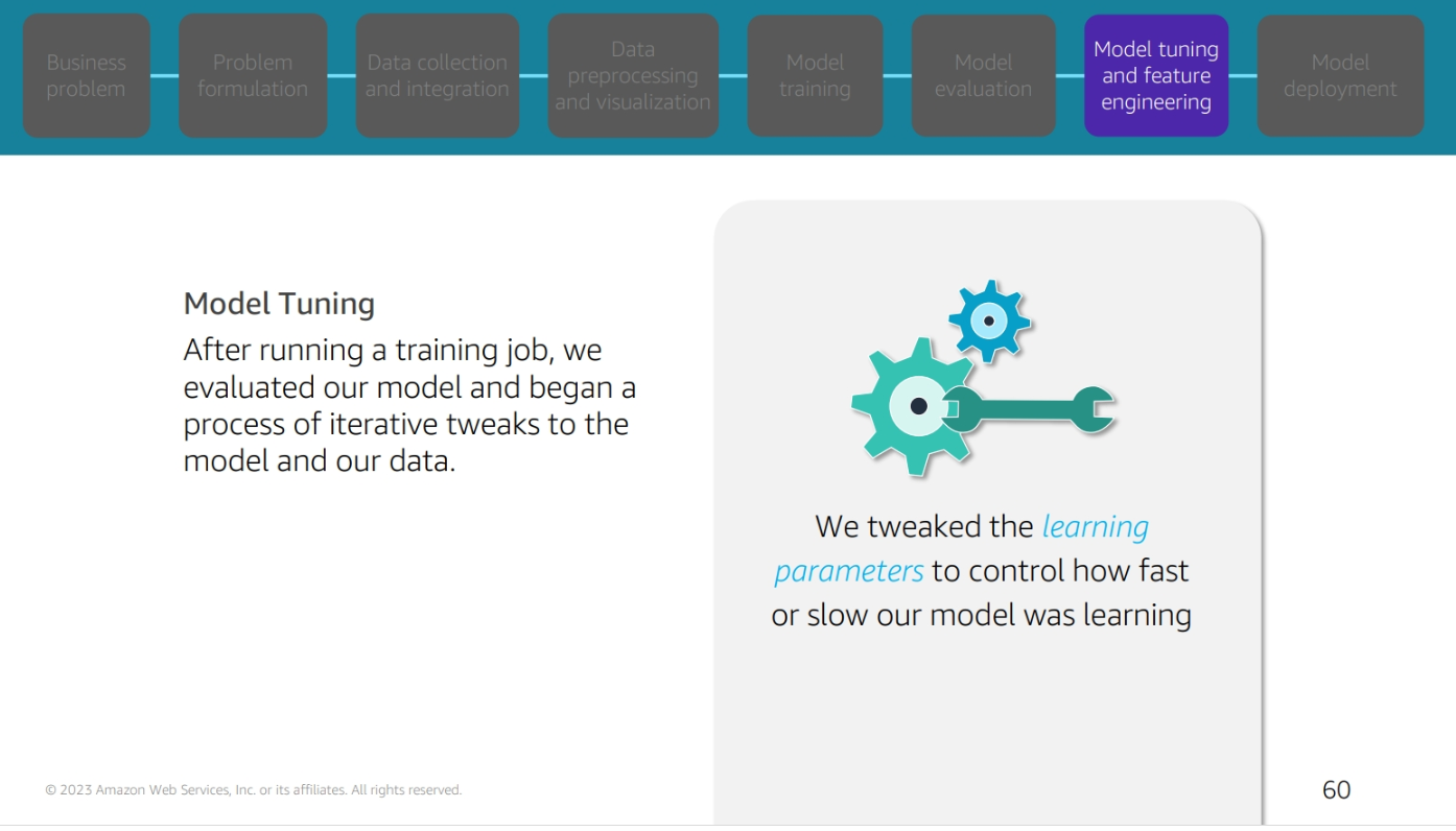
Model tuning and feature enginnering

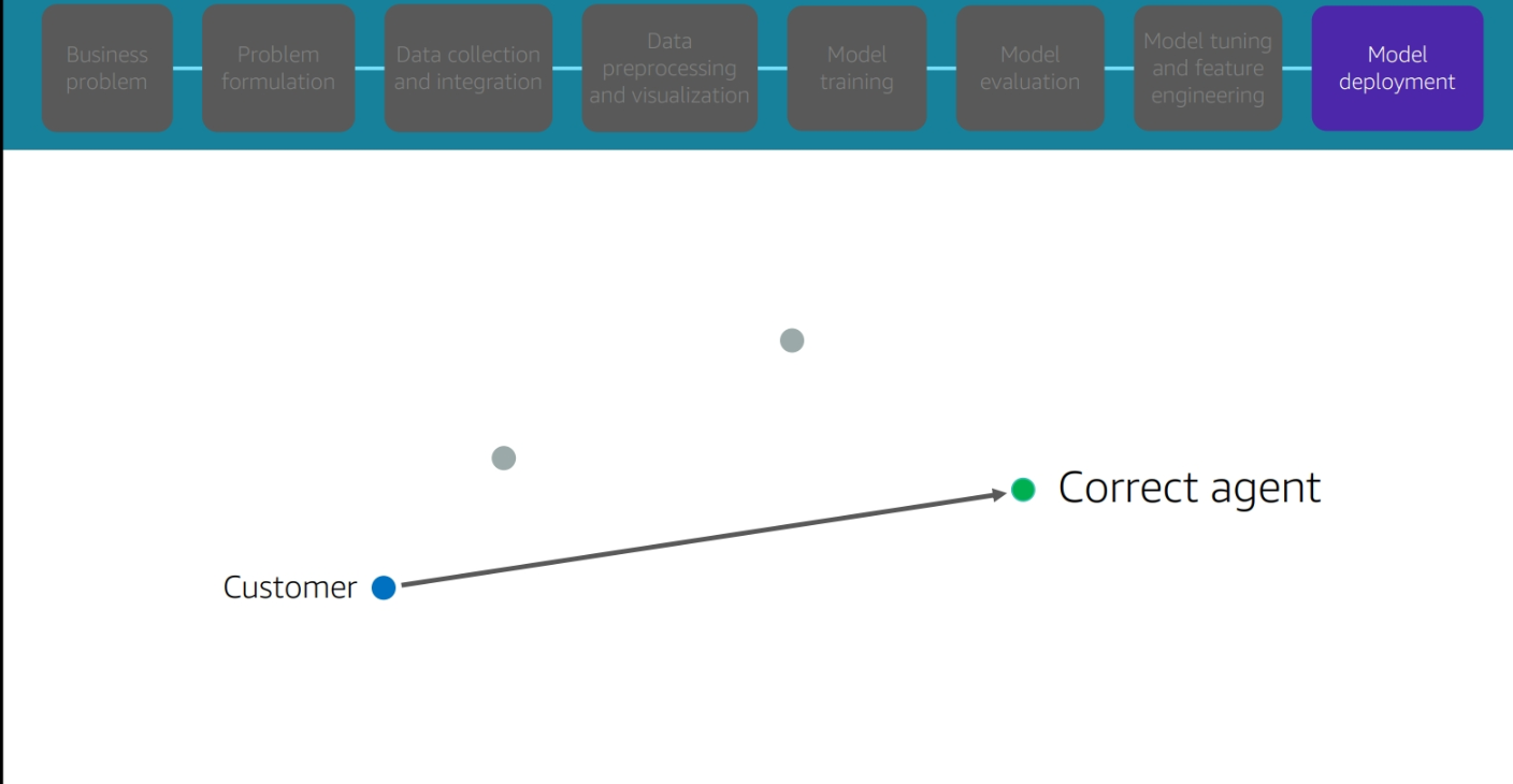
Model deployment

Module 2: AWS SageMaker

Amazon SageMaker is a fully-managed service used to build, train and deploy ML models at any scale. You can use part or all of Amazon SageMaker features.

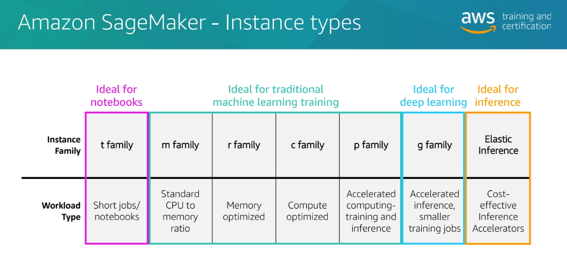
Instances Types

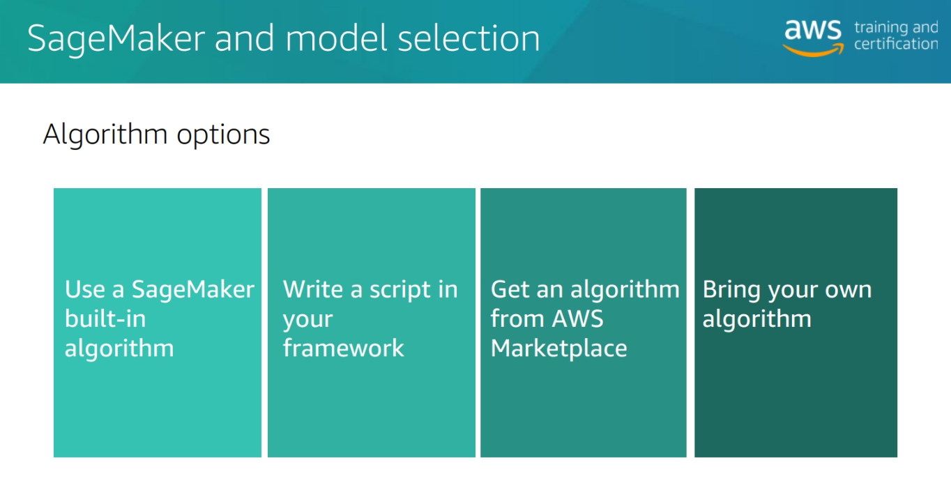
Algorithm options

SageMaker Deploytme

Module 3 : Problem Formulation

Problem Formulation

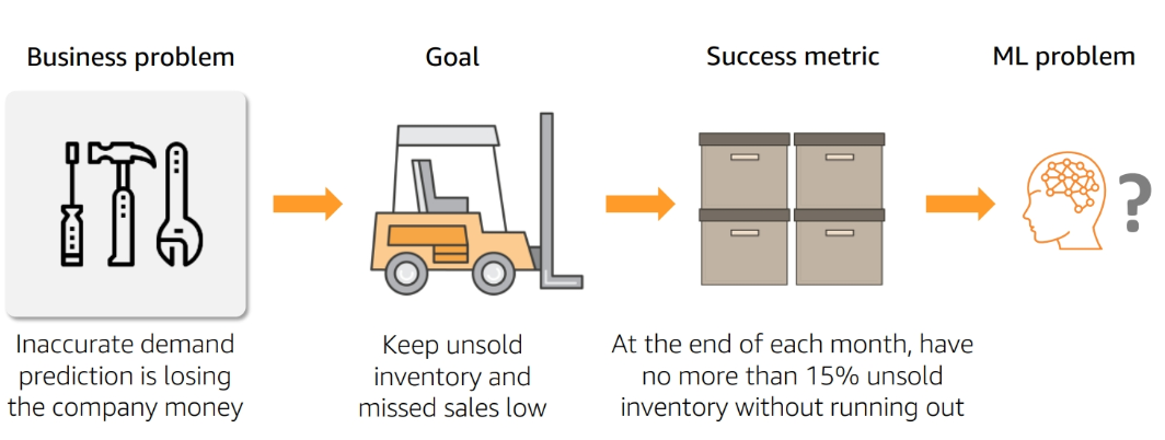
Define Success

Model Performance metrics:
- Example: The model should have an accuracy of 90% in predicting whether a customer will buy a Kindle
  - Accuracy
  - Precision
  - Recall
  - F1 score
  - AUC
Business Metrics:
- Example: The model should increase the number of Kindles sold by 10%
  - Revenue
  - Customer satisfaction
  - Customer retention
  - Customer acquisition

Module 4: Data Preoprocessing

Python libraries for data preprocessing

Pandas: Data manipulation and analysis which provides data structures and functions to manipulate numerical tables and time series data.

import pandas as pd

Numpy: A library for the Python programming language, adding support for large, multi-dimensional arrays and matrices, along with a large collection of high-level mathematical functions to operate on these arrays.

import numpy as np

Matplotlib: A plotting library for the Python programming language and its numerical mathematics extension NumPy.

import matplotlib.pyplot as plt

Seaborn: A Python data visualization library based on matplotlib. It provides a high-level interface for drawing attractive and informative statistical graphics.

import seaborn as sns

Statistics for data preprocessing

Mean: The average of the numbers
Median: The middle number
Mode: The number that appears most often
Standard Deviation: A measure of the amount of variation or dispersion of a set of values
Variance: A measure of the amount of variation or dispersion of a set of values
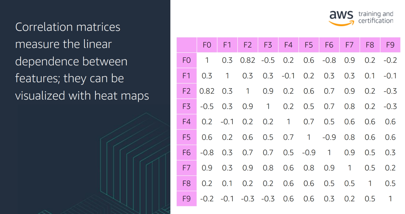
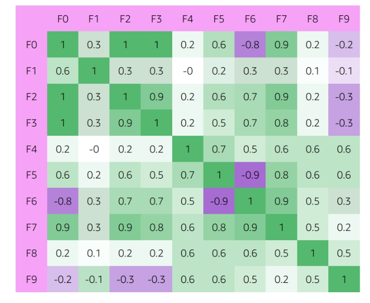
Correlation: A measure of the strength and direction of the relationship between two variables
Covariance: A measure of the relationship between two random variables

Dealing with outliers

Outliers: An observation that lies an abnormal distance from other values in a random sample from a population
Aritificial Outliers: Outliers that are created by errors in data collection or entry
Natural Outliers: Outliers that are part of the population
- ** Tranformation**: Logarithmic, square root, cube root, reciprocal, square, cube, exponential, and power transformations
- ** impute a value**: Replace the outlier with a value that is within the range of the data
Methods to detect outliers:
- Boxplot
- Z-score
- IQR score
- Scatter plot
- Histogram
- DBSCAN
- Isolation Forest
- Local Outlier Factor
- Elliptic Envelope
- One-Class SVM

Module 5: Model Training

Overfitting and Underfitting and Balanced

Overfitting: The model is too complex and learns the training data too well
Underfitting: The model is too simple and does not learn the training data well
Balanced: The model learns the training data well and generalizes to new data

Bias and Variance

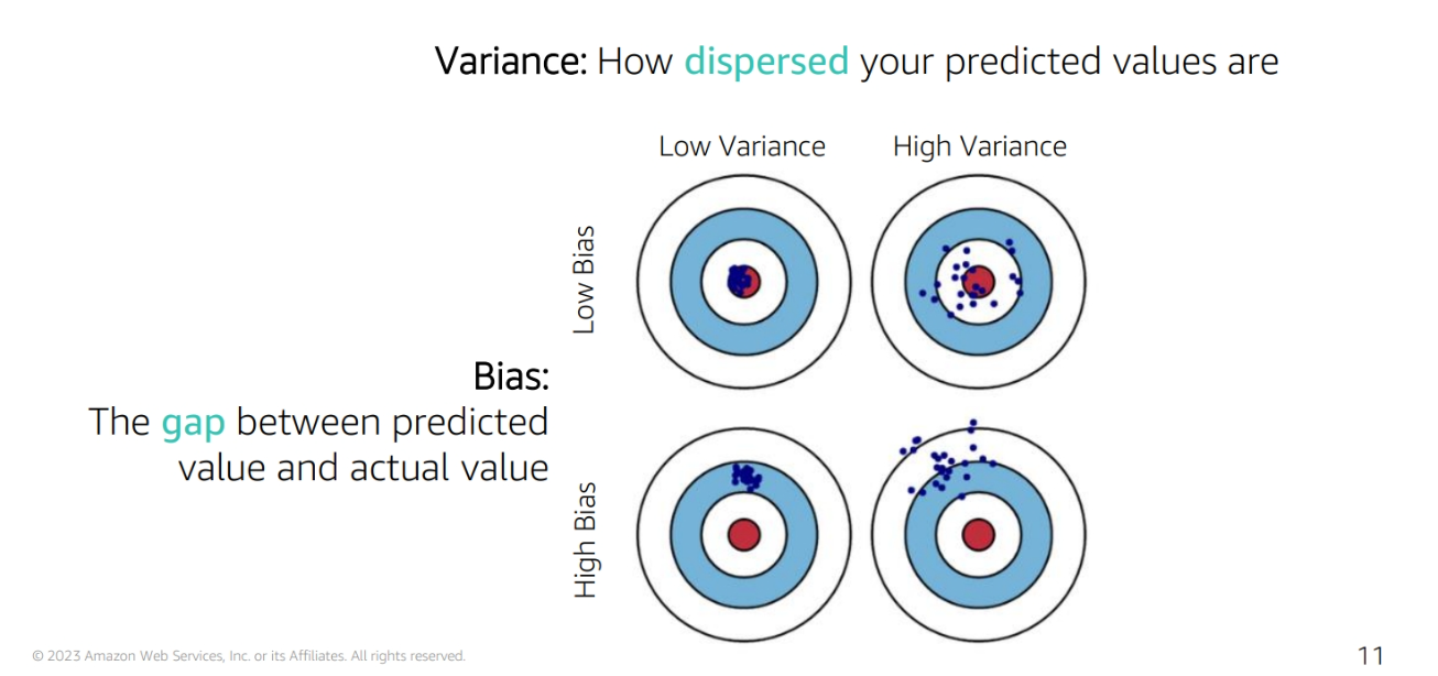
Bias: The error introduced by approximating a real-world problem, which may be extremely complicated, by a much simpler model
Variance: The error introduced by attempting to approximate a real-world problem by a much simpler model

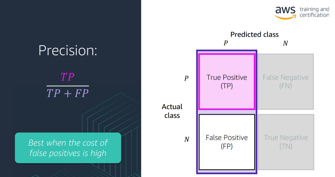
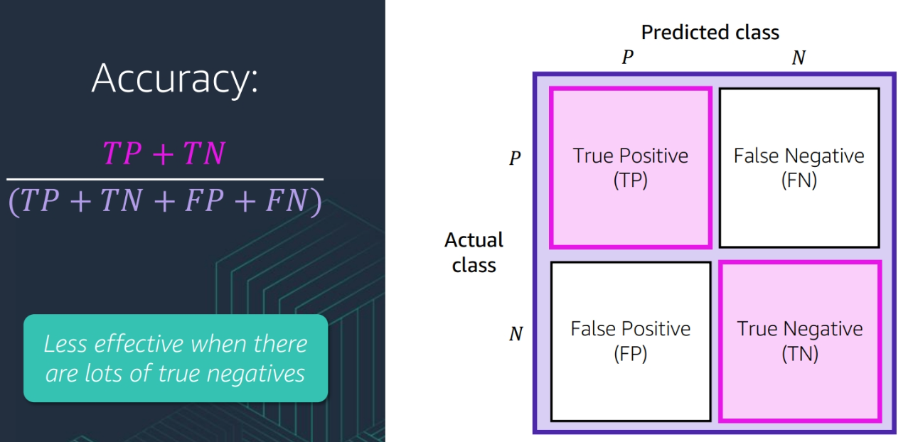
Confusion Matrix

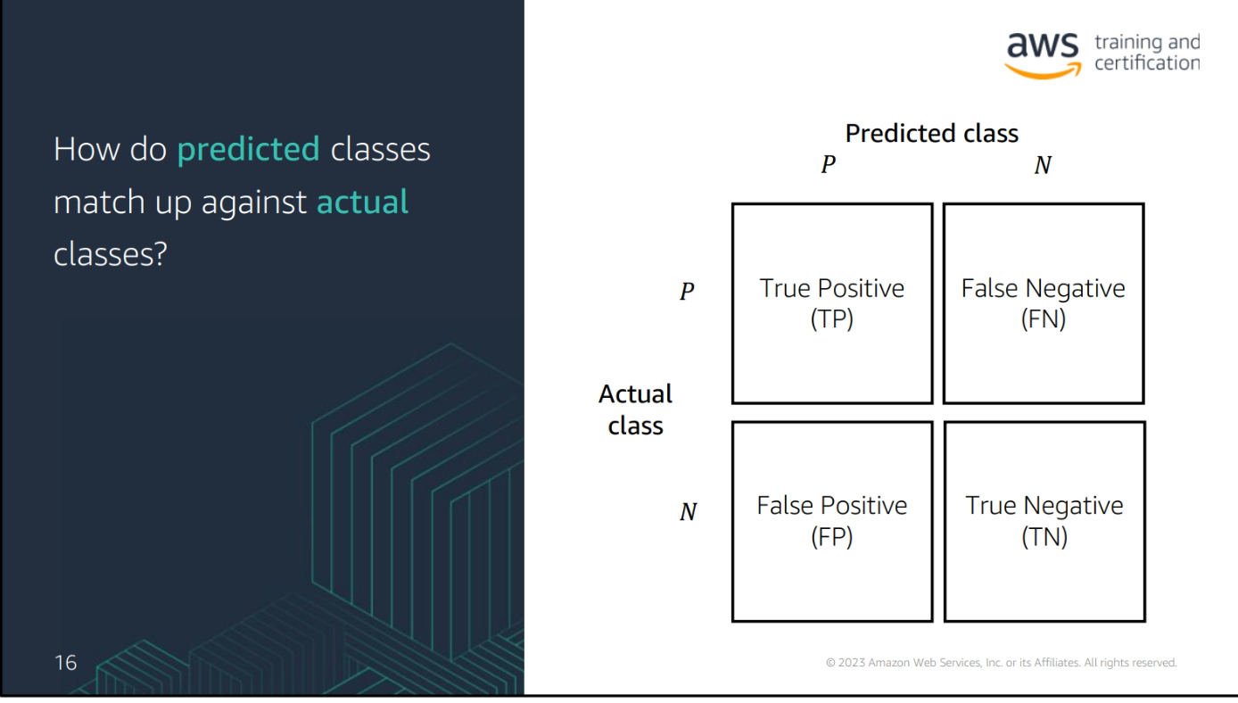
True Positive (TP): The number of positive cases that were correctly predicted
True Negative (TN): The number of negative cases that were correctly predicted
False Positive (FP): The number of negative cases that were incorrectly predicted as positive
False Negative (FN): The number of positive cases that were incorrectly predicted as negative

Precision, Recall, F1 Score, and AUC

Precision: The number of true positive cases divided by the number of true positive and false positive cases (TP / (TP + FP))

Accuracy: The number of true positive and true negative cases divided by the total number of cases (TP + TN) / (TP + TN + FP + FN)

Recall: The number of true positive cases divided by the number of true positive and false negative cases (TP / (TP + FN))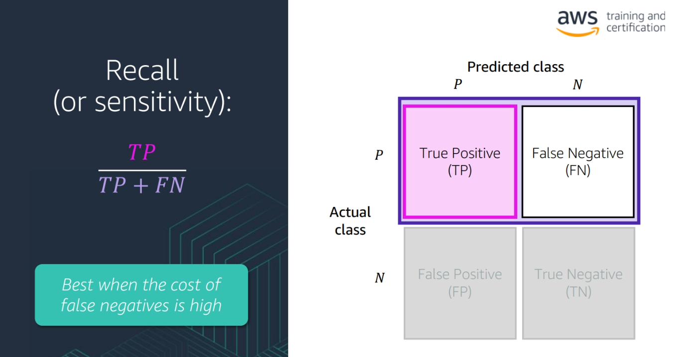
F1 Score: The harmonic mean of precision and recall 2 * (precision * recall) / (precision + recall)
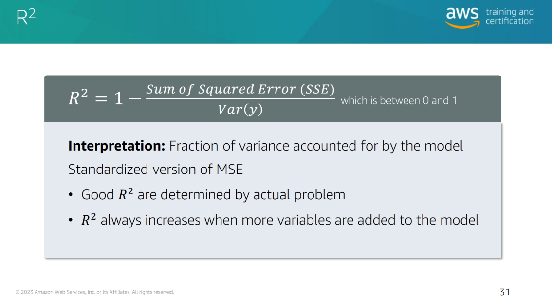
AUC: The area under the receiver operating characteristic curve, which is a plot of the true positive rate against the false positive rate
ROC Curve: A plot of the true positive rate against the false positive rate
AUC-ROC curve is a performance measurement for classification problem at various threshold settings. ROC is a probability curve and AUC represents degree or measure of separability. It tells how much model is capable of distinguishing between classes. Higher the AUC, better the model is at predicting 0s as 0s and 1s as 1s. By analogy, the Higher the AUC, the better the model is at distinguishing between patients with disease and no disease.

Types of Problems Score

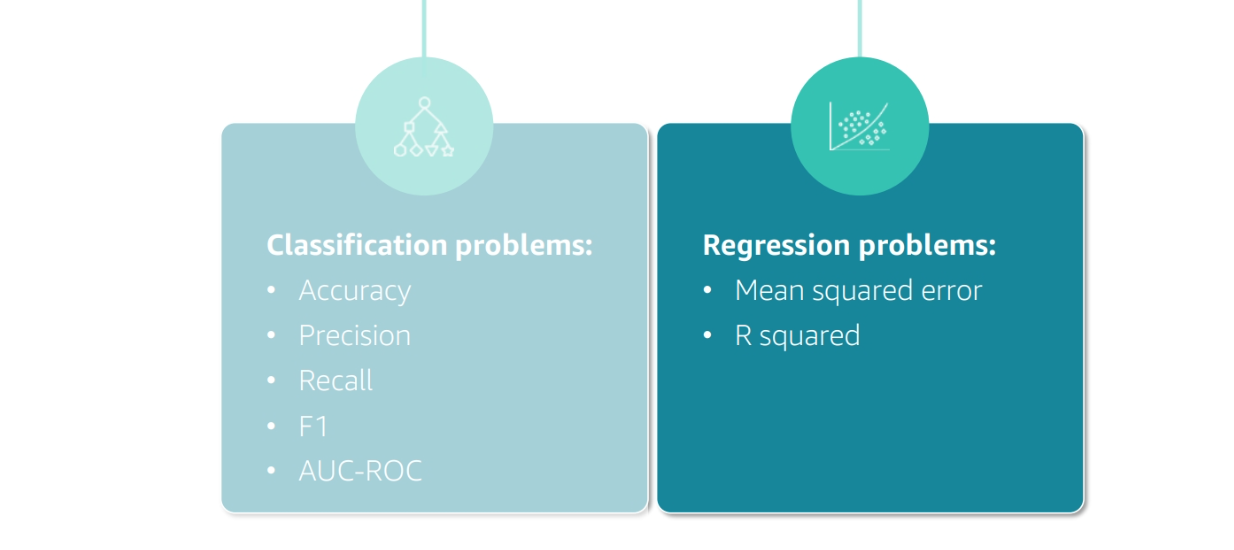
R2

Module 7: Model Tuning and Feature Engineering

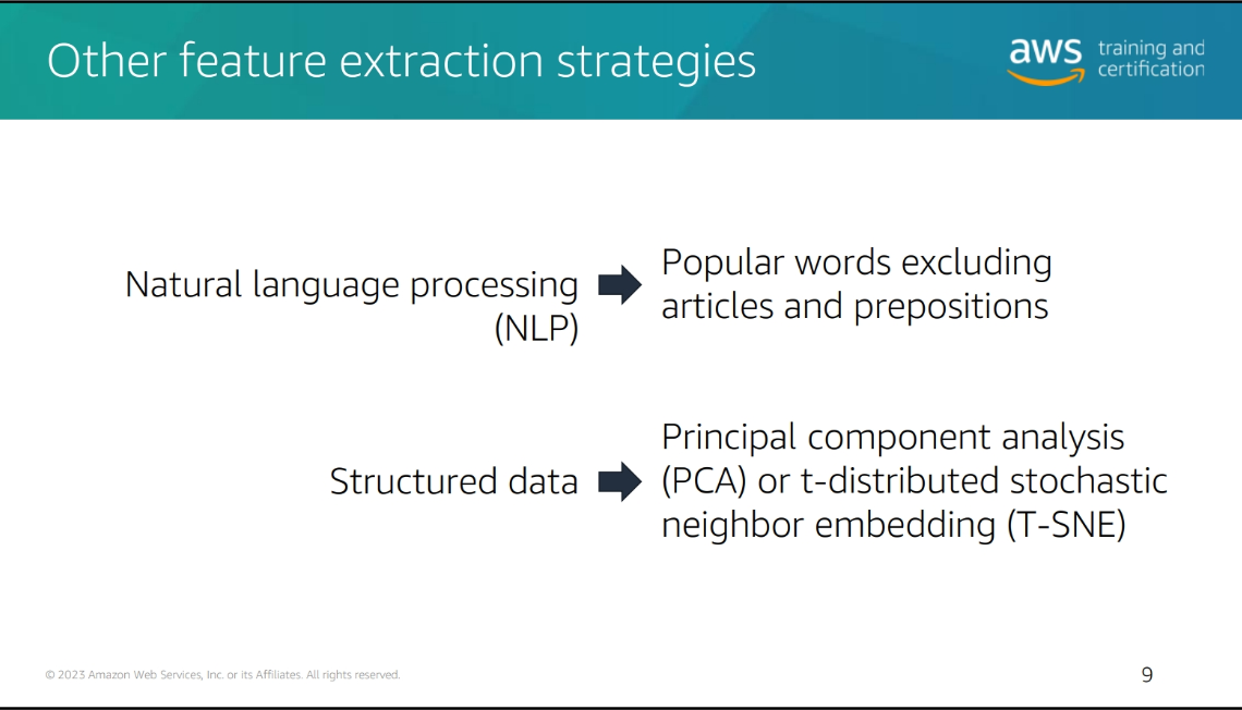
Feature Engineering components

Feature Selection: Selecting the most important features
Feature Extraction: Extracting new features from existing features
Feature Transformation: Transforming features to improve model performance
Feature Scaling: Scaling features to improve model performance

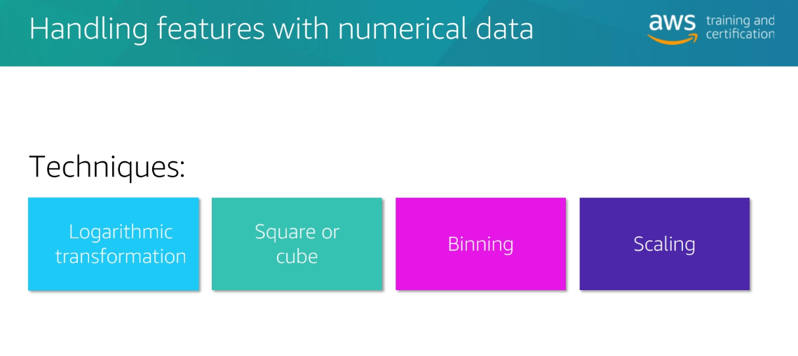
Techniques

Why we choose feature engineering

Improve model performance: Feature engineering can improve the performance of a model
Reduce overfitting: Feature engineering can reduce overfitting by removing irrelevant features
Reduce underfitting: Feature engineering can reduce underfitting by adding relevant features
Improve interpretability: Feature engineering can improve the interpretability of a model by creating features that are easier to understand

Why change numerical to small number

Reduce computational cost: Smaller numbers require less memory and less computation
** Make the model more aware of the scale of the data**: The model will be more aware of the scale of the data and will be able to learn more effectively

Note : so the model think that the small number is more important than the large number

why change numerical to categorical

make more sense to the model example: Age: 0-18, 19-30, 31-50, 51-70, 71-100 This will make more sense to the model than the original numerical data

Scaling transformation techniques

Min-Max Scaling: Scales the data to a fixed range, usually 0 to 1
Standardization: Scales the data to have a mean of 0 and a standard deviation of 1
Max Abs Scaling: Scales the data to a fixed range, usually -1 to 1 or 0 to 1
Normalization: Scales the data to have a magnitude of 1

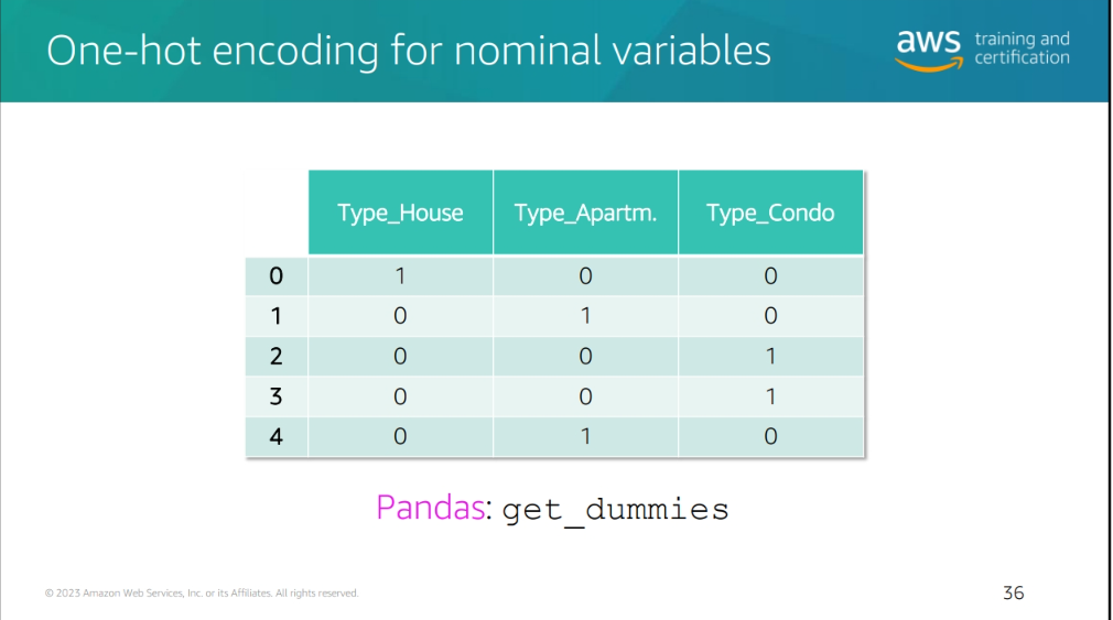
one hot encoding

One-Hot Encoding: A method of converting categorical data into a format that can be provided to ML algorithms to do a better job in prediction. It is a process of converting categorical data into a binary matrix format.

sometimes it's not efficient to do this so you could try

**Group By somthing Similar

Hyperparameter Tuning

Hyperparameters: Parameters that are set before the model is

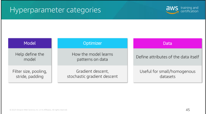
Hyperparameter Tuning seearch methods

Grid Search: A method of hyperparameter tuning that searches through a specified subset of hyperparameters
Random Search: A method of hyperparameter tuning that searches through a random subset of hyperparameters
Bayesian Optimization: A method of hyperparameter tuning that uses a probabilistic model to search through a subset of hyperparameters

Model 8 Model Deployment

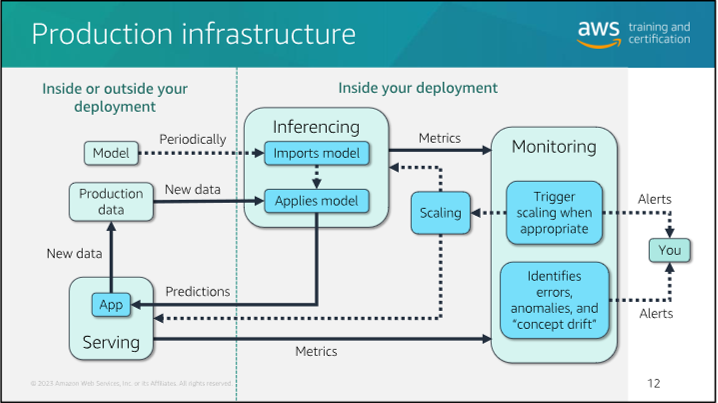
Types of inferences

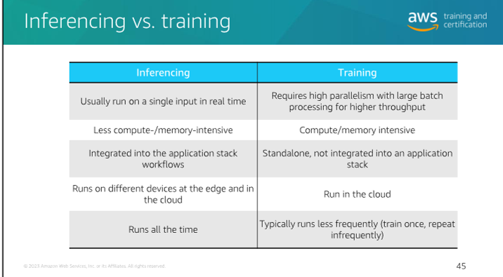
Inferecing vs. Training

Blue-Green Deployment and Canary Deployment:
- Blue-Green Deployment:
  - What is it? Blue-green deployment is a release management strategy used in software deployment. It involves maintaining two identical production environments: one called "Blue" (the active environment) and the other "Green" (the inactive environment).
  - How does it work?
    1. Preparation: Set up a staging environment (Green) that mirrors the production environment (Blue).
    2. Deployment: Deploy the new version of your application to the inactive environment (Green).
    3. Testing: Thoroughly test the new version in the inactive environment to ensure stability.
    4. Switch: Once confident, switch users to the Green environment, making it the new active production environment.
  - Goal: Minimize downtime and reduce risk during software updates.
- Canary Deployment:
  - What is it? Canary deployment gradually rolls out new software versions to a controlled subset of users before deploying to everyone.
  - How does it work?
    1. Incremental Rollout: Deploy the new version to a percentage of users (the "canaries").
    2. Monitoring: Monitor canaries' feedback and performance.
    3. Iterate: Address any issues that arise. If successful, proceed with a full-scale release.
  - Goal: Identify and fix issues early, minimizing widespread problems or outages.
Amazon SageMaker:
- What is it? Amazon SageMaker is a fully managed machine learning (ML) service provided by AWS.
- Features:
  - Build, Train, and Deploy: Data scientists and developers can build, train, and deploy ML models in a production-ready hosted environment.
  - UI Experience: SageMaker provides a user-friendly interface for ML workflows across multiple integrated development environments (IDEs).
  - Managed ML Algorithms: Efficiently run ML algorithms against large data in a distributed environment.
  - Flexible Training Options: Supports custom algorithms and frameworks.
  - Secure and Scalable Deployment: Easily deploy models from the SageMaker console.
- Use Cases: SageMaker is ideal for various ML tasks, including image classification, natural language processing, and time series forecasting.
- Point Clouds and SageMaker:
  - Amazon SageMaker Ground Truth simplifies labeling objects in 3D point clouds for ML training datasets.
  - It supports sensor fusion of camera and LiDAR data, making it useful for applications like autonomous vehicles.

Checkout

https://stanford-cs329s.github.io/syllabus.html